Geometry Objects: Representation, Parametrization, and Mapping

Why geometries in CUQIpy?

Geometry objects in CUQIpy serve two main purposes:

1. They simplify visualization by embedding plotting tools directly within the arrays and objects, such as CUQIArrays and Samples. This is demonstrated throughout the book using methods like plot.

2. They provide a mapping between parameter vectors and function values, enabling CUQIpy’s sampling algorithms (operating on vectors) to be compatible with more complex representations like 2D images.

Parametrization and Mapping with Geometries

One way to view the Geometry object is as a parameter-to-function mapping (and sometimes also a function-to-parameter mapping). The function space is what the forward models are operating on, e.g. a 2D convolution on images, while the parameter space is what the sampling algorithms are operating on. These mappings can also be more complicated, such as a mapping coefficients of an expansion to the function values on a PDE mesh.

A vector of values (unknown parameters or data) in the Bayesian Inverse problem setting can be interpreted in various ways. It can be, for example, a vector of function values at 1D or 2D grid points, a vector of image pixels, a vector of expansion coefficients, or a collection of variables, e.g. the temperature measurement at four cities: A, B, C, and D.

In CUQIpy, the cuqi.geometry module provides classes for different representations of vectors, e.g Continuous1D, Continuous2D, Image2D, and Discrete.

Here we explore geometry assignment for Distributions, Samples and CUQIarray. We explore the three main functionalities of the geometry objects: representation, parametrization, and mapping.

Variable representation

First let us create 1000 samples from a 4-element distribution \(y\):

Show code cell content Hide code cell content

from cuqi.distribution import Gaussian
from cuqi.geometry import Image2D, Discrete, StepExpansion, MappedGeometry
from cuqi.array import CUQIarray
import numpy as np

mu = np.array([5, 3, 1, 0])
sigma = np.array([1, 2, 3, 0.5])
y = Gaussian(mean=mu, cov=sigma**2)
y_samples = y.sample(1000)

If no geometry is provided by the user, when creating a Distribution for example, CUQIpy will assign _DefaultGeometry1D (trivial geometry) to the distribution and the Samples produced from it.

print(y.geometry)
print(y_samples.geometry)

_DefaultGeometry1D(4,)
_DefaultGeometry1D(4,)

Samples are plotted with line plot by default, which is due to how the _DefaultGeometry1D interprets the samples.

y_samples.plot([100,200,300])

[<matplotlib.lines.Line2D at 0x7fc5a1cddc30>,
 <matplotlib.lines.Line2D at 0x7fc5a1cddd20>,
 <matplotlib.lines.Line2D at 0x7fc5a1cdde10>]

We may equip the distribution with a different geometry, either when creating it, or afterwards. Let us for example assign an Image2D geometry to the distribution y. First we create the Image2D geometry and we assume the shape of the image is \(2\times2\):

geom_image = Image2D((2,2))
print(geom_image)

Image2D(4,)

We can check the number of parameters (parameter dimension) of the geometry:

geom_image.par_dim

4

We can also check the shape of its representation (size of the image in this case) using the property fun_shape:

geom_image.fun_shape

(2, 2)

Now we equip the distribution y with this Image2D geometry.

y.geometry = geom_image

Check the geometry of y:

y.geometry

Image2D(4,)

With this distribution set up, we are ready to generate some samples

# call method to sample
y_samples = y.sample(50)

We can check that we have produced 50 samples, each of size 4:

y_samples.shape

(4, 50)

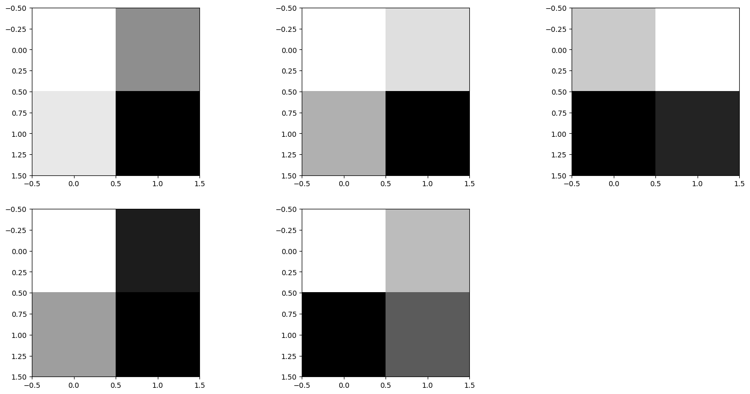
We plot a couple of samples:

y_samples.plot()   

Plotting 5 randomly selected samples

[<matplotlib.image.AxesImage at 0x7fc5a1d99420>,
 <matplotlib.image.AxesImage at 0x7fc5a1dd2710>,
 <matplotlib.image.AxesImage at 0x7fc59fc3d9c0>,
 <matplotlib.image.AxesImage at 0x7fc59fc3f310>,
 <matplotlib.image.AxesImage at 0x7fc59fca7280>]

What if the 4 parameters in samples have a different meaning? For example, the four parameters might represent labelled quantities such as temperature measurement at four cities A, B, C, D. In this case, we can use a Discrete geometry:

geom_discrete = Discrete(['Temperature A', 'Temperature B', 'Temperature C', 'Temperature D'])
print(geom_discrete)

Discrete(4,)

We can update the distribution’s geometry and generate some new samples:

y.geometry = geom_discrete

y_samples = y.sample(100)

The samples will now know about their new Discrete geometry and the plotting style will be changed:

y_samples.plot();

Plotting 5 randomly selected samples

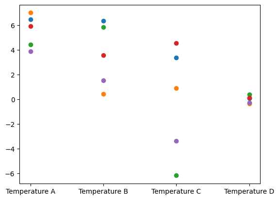
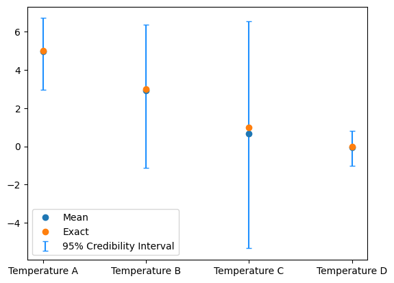
The credibility interval plot style is also updated to show errorbars for the Discrete geometry:

y_samples.plot_ci(95, exact=mu)

[<matplotlib.lines.Line2D at 0x7fc59efdefe0>,
 <matplotlib.lines.Line2D at 0x7fc59f0009a0>,
 <ErrorbarContainer object of 3 artists>]

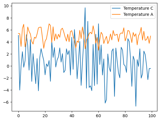
And similarly, in the chain plot, the legend reflects the particular labels:

y_samples.plot_chain([2,0])

[<matplotlib.lines.Line2D at 0x7fc59fa099f0>,
 <matplotlib.lines.Line2D at 0x7fc59fa09ae0>]

Varible parameterization

In CUQIpy we have geometries that represents a particular parameterization of the variables (e.g. StepExpansion, KLExpansion, etc). For example, in the StepExpansion geometry, the parameters represent expansion coefficients for equidistance-step basis functions. You can read more about StepExpansion by typing help(cuqi.geometry.StepExpansion) in a the code cell below or by looking at the documentation of StepExpansion

Let us create a StepExpansion geometry, we first need to create a grid on which the step functions are defined, let us assume the grid is defined on the interval \([0,1]\):

grid = np.linspace(0, 1, 100)

Then we create the StepExpansion geometry with 4 steps and assign it to the distribution y:

geom_step_expantion = StepExpansion(grid, n_steps=4)
y.geometry = geom_step_expantion
print(y.geometry)

StepExpansion(4,)

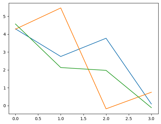
Let us samples the distribution y and plot the samples:

y_step_samples = y.sample(100)
y_step_samples.plot()

Plotting 5 randomly selected samples

[<matplotlib.lines.Line2D at 0x7fc59fa93250>,
 <matplotlib.lines.Line2D at 0x7fc59fa93340>,
 <matplotlib.lines.Line2D at 0x7fc59fa93430>,
 <matplotlib.lines.Line2D at 0x7fc59fa93520>,
 <matplotlib.lines.Line2D at 0x7fc59fa920b0>]

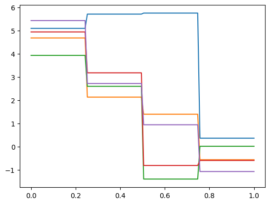
Note that the samples are now represented as expansion coefficients of the step functions.

Examples of using StepExpansion and KLExpansion geometries in the context of a PDE parameterization for a heat 1D BIP can be found here, and here [ARA+24], respectively.

Variable mapping

In CUQIpy, we provide the MappedGeometry object which equips geometries with a mapping function that are applied to the variables, this mapping can also be viewed as parametrization. An example of a commonly used mapping in inverse problems is \(e^x\) for unknown parameters \(x\) to ensure positivity regardless of the value of \(x\).

Let us use the MappedGeometry to map the StepExpansion geometry we created earlier with the exponential function:

geom_step_expantion_mapped = MappedGeometry(geom_step_expantion, map=lambda x: np.exp(x))

Let us again, assign the MappedGeometry to the distribution y and generate samples and plot them:

y.geometry = geom_step_expantion_mapped
y_mapped_step_samples = y.sample(100)
y_mapped_step_samples.plot()

Plotting 5 randomly selected samples

[<matplotlib.lines.Line2D at 0x7fc59f92a3e0>,
 <matplotlib.lines.Line2D at 0x7fc59f92a4d0>,
 <matplotlib.lines.Line2D at 0x7fc59f92a5c0>,
 <matplotlib.lines.Line2D at 0x7fc59f92a6b0>,
 <matplotlib.lines.Line2D at 0x7fc59f92a7a0>]

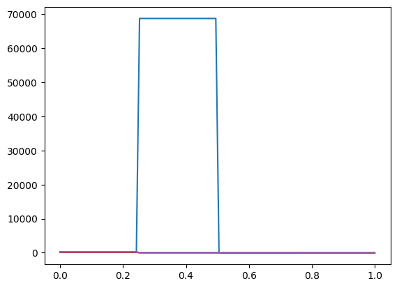
Note that the samples are still representing the expansion coefficients of the step functions, but the mapping function \(e^x\) has been applied to the samples. All samples are now non-negative.

★ Elaboration: Specifying a Geometry object for CUQIarray objects:

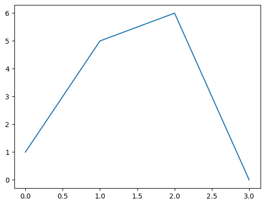
Geometries can also be specified for CUQIarray, the basic array structure in CUQIpy. Let us create a CUQIarray object with four parameters as follows:

q = CUQIarray([1,5,6,0])

We look at the geometry property

q.geometry

_DefaultGeometry1D(4,)

And then let us plot our variable q:

q.plot()

[<matplotlib.lines.Line2D at 0x7fc59f9b9d50>]

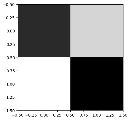
We now choose a different interpretation for the variable q by changing its geometry to, for example, the Image2D geometry we created, and then we plot:

q.geometry = geom_image
q.plot()

[<matplotlib.image.AxesImage at 0x7fc59f803190>]

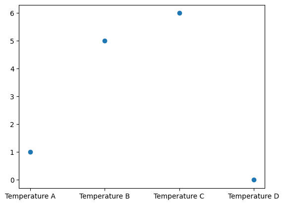
Finally we set the Discrete geometry we created as the geometry for q and plot:

q.geometry = geom_discrete
q.plot()

[<matplotlib.lines.Line2D at 0x7fc59f8c1960>]