\(\gdef\dd{\mathrm{d}}\)
\(\gdef\abs#1{\left\vert#1\right\vert}\)
\(\gdef\ve#1{\bm{#1}}\)
\(\gdef\mat#1{\mathbf{#1}}\)
Two forward models#
We introduce here two forward models: 1D Poisson and 1D convolution. We will use these forward models in the book to apply and demonstrate various concepts in Bayesian inversion.
Contents of this notebook: #
Learning objectives: #
Create (or load pre-existing) linear and non-linear forward models in CUQIpy and use them
Create and plot input for the forward models and compute and plot the corresponding output
Mathematically define two forward models: 1D Poisson and 1D Convolution and use them in CUQIpy
Show code cell content
from cuqi.testproblem import Poisson1D, Deconvolution1D, Heat1D
from cuqi.distribution import Gaussian
from cuqi.array import CUQIarray
import numpy as np
import matplotlib.pyplot as plt
Forward model: 1D Poisson #
Consider a heat conductive rod of length \(L = \pi\) with a varying conductivity (the conductivity of the rod changes from point to point). We fix the temperature at the end-points of the rod and apply a heat source distributed along the length of the rod. We wait until the rod reaches an equilibrium temperature distribution. The equilibrium temperature of the rod is modelled using the second order steady-state PDE as
Here, \(y\) represents the temperature distribution along the rod, \(u(\xi) \) is the unknown conductivity of the rod and \(f(\xi)\) is a deterministic heat source given by
To ensure that the conductivity of the rod is non-negative, we parameterize \(u\) by a random variable \(x\) as follows:
where \(x\) is not necessarily positive.
Let us load the forward model that maps the random variable \(x\) to the temperature distribution \(y\) in CUQIpy. We will use the following parameters:
dim: number of discretization points for the rodL: length of the rodf: a function that represents the heat source
dim = 128
L = np.pi
f = lambda xi: 10*np.exp(-(xi-L/2)**2 / 0.02)
Then we can load the 1D Poisson forward model as follows:
A = Poisson1D(dim=dim, endpoint=L, source=f).model
We print the forward model to see its details.
A
CUQI PDEModel: Continuous1D(128,) -> Continuous1D(127,).
    Forward parameters: ['x'].
    PDE: SteadyStateLinearPDE.
We can look at the domain and range geometries of the forward model.
print(A.domain_geometry)
print(A.range_geometry)
Continuous1D(128,)
Continuous1D(127,)
These geometries are of type Continuous1D which represents a 1D continuous signal/field defined on a grid. We can view the grid:
print(A.domain_geometry.grid)
[0.         0.02473695 0.0494739  0.07421085 0.0989478  0.12368475
 0.1484217  0.17315865 0.1978956  0.22263255 0.2473695  0.27210645
 0.2968434  0.32158035 0.3463173  0.37105425 0.3957912  0.42052815
 0.4452651  0.47000205 0.494739   0.51947595 0.5442129  0.56894985
 0.5936868  0.61842375 0.6431607  0.66789765 0.6926346  0.71737155
 0.7421085  0.76684545 0.7915824  0.81631935 0.8410563  0.86579325
 0.8905302  0.91526715 0.9400041  0.96474105 0.989478   1.01421495
 1.0389519  1.06368885 1.0884258  1.11316275 1.1378997  1.16263665
 1.1873736  1.21211055 1.2368475  1.26158445 1.2863214  1.31105835
 1.3357953  1.36053225 1.3852692  1.41000615 1.4347431  1.45948005
 1.484217   1.50895395 1.5336909  1.55842785 1.5831648  1.60790175
 1.6326387  1.65737565 1.6821126  1.70684955 1.7315865  1.75632345
 1.7810604  1.80579735 1.8305343  1.85527125 1.8800082  1.90474515
 1.9294821  1.95421905 1.978956   2.00369295 2.0284299  2.05316685
 2.0779038  2.10264075 2.1273777  2.15211465 2.1768516  2.20158855
 2.2263255  2.25106245 2.2757994  2.30053635 2.3252733  2.35001025
 2.3747472  2.39948415 2.4242211  2.44895805 2.473695   2.49843195
 2.5231689  2.54790585 2.5726428  2.59737975 2.6221167  2.64685365
 2.6715906  2.69632755 2.7210645  2.74580145 2.7705384  2.79527535
 2.8200123  2.84474925 2.8694862  2.89422315 2.9189601  2.94369705
 2.968434   2.99317095 3.0179079  3.04264485 3.0673818  3.09211875
 3.1168557  3.14159265]
Additionally, the properties domain_dim and range_dim of the forward model represent the dimension of the input and output of the forward model, respectively.
print(A.domain_dim)
print(A.range_dim)
128
127
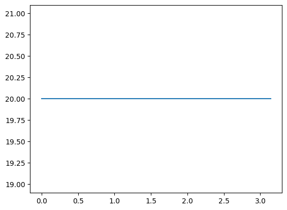
Let us create an array representing a constant conductivity over the grid nodes
some_x_array = 20*np.ones(A.domain_dim)
We can wrap the array in a CUQIarray object which is the main data structure in CUQIpy for variables (e.g. arrays and fields)
some_x = CUQIarray(some_x_array, geometry=A.domain_geometry)
Note that we pass geometry=A.domain_geometry to equip the CUQIarray object with the same geometry as the domain of the forward model, which is has information about what the values of the array represent (e.g. function values on a grid for this case).
We can plot the conductivity array using the plot method of the CUQIarray object
some_x.plot()
[<matplotlib.lines.Line2D at 0x7f88f8e61d20>]
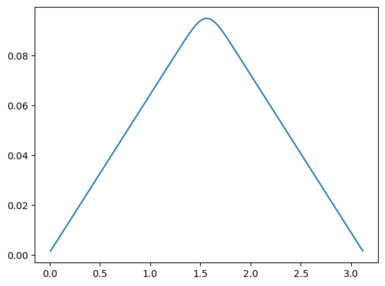
We can also evaluate the forward model at the conductivity array and plot the solution:
some_y = A(some_x)
some_y.plot()
[<matplotlib.lines.Line2D at 0x7f88f8d4a950>]
Exercise: #
Is this true for you: “I can, mathematically, write a definition of a 1D Poisson forward model that maps the conductivity field to the temperature distribution field”? If not, what questions do you have?
Trying a different conductivity profile:
Create another constant conductivity profile
another_xof value 20 as aCUQIarrayobject.Evaluate the forward model at the new conductivity profile and store the result in a variable
another_y. Plot the solution.In one plot, compare the solutions
some_yandanother_yusing theplotmethod of theCUQIarrayobject. What do you observe? and why?
Experimenting with setting up the
mapinPoisson1D:Execute
help(Poisson1D)Note the
mapparameter ofPoisson1D. We can use this parameter to transform the conductivity field before solving the PDE. Create the forward model again, name itA_map, with setting upmapto belambda x: np.exp(x)to ensure that the conductivity is always positive.Inspect the domain and range geometries of the new forward model
A_mapwhat is different this time, and why?Create a CUQIarray object
x_with_mapwith a constant conductivity profile of value 0 and evaluate the forward model atx_with_mapand store it in variabley_with_map. Make sure to use the right geometry forx_with_map.Plot
x_with_mapusingx_with_map.plot(), What do you observe?Plot the solution
y_with_mapandsome_yin the same plot. What do you observe? and why?
Experimenting with setting up the
field_typeinPoisson1D:Note the
field_typeparameter ofPoisson1D. We can use this parameter to change the parameterization of the conductivity field. Create the forward model again, name itA_step, with setting both themapas in the previous exercise and thefield_typeto be"Step"to generate a step parameterization of the conductivity field.What is the domain and range geometries of the new forward model
A_step?Create
x_stepto bex_step = CUQIarray(np.arange(A_step.domain_dim)*0.1, geometry=A_step.domain_geometry).Plot
x_stepusingx_step.plot().What does the dimension
A_step.domain_dimrepresent? and is it equal to the size of the domain geometry grid?Evaluate the forward model at
x_stepand store it in variabley_step. Plot the solution.
Is this true for you: “I can load the pre-existing Poisson 1D forward model in CUQIpy and evaluate it on some input and visualize the input and output”? If not, what questions do you have?
# your code here
Forward model: 1D convolution #
The mathematical model for convolution of a random signal on a one-dimensional spatial domain \(D\), can be written as a stochastic Fredholm integral equation of the first kind:
where \(y(\xi)\) denotes the convolved signal and we assume a Gaussian convolution kernel. In practice, a finite-dimensional representation of the integral equation is employed. After discretizing the signal domain into \(N\) components, the convolution model can be expressed as a system of linear algebraic equations \(\ve{y}=\mat{K}\ve{x}\).
Let us load the forward model that maps the random variable \(\ve{x}\) to the convolved signal \(\ve{y}\) in CUQIpy. We will use the following parameters to specify the forward model:
dim: is the number of discretization points for the signal, \(N\)PSF: a function that represents the point spread function, i.e., the convolution kernelPSF_size: the size of the PSF (less or equal todim)PSF_param: A parameter of the PSF, the larger the size the more the blur applied to the signalBC: boundary conditions for the convolution
We set the parameters as follows:
dim = 201
PSF = 'gauss' # Gaussian PSF
PSF_size = np.round(dim/3)
PSF_param = np.round(dim/20)
BC='reflect' # Boundary condition
Then we can load the 1D convolution forward model as follows (note that we refer to the forward model as a convolution model which we obtain from the Deconvolution1D test problem, the latter represents the BIP of deconvolving the signal):
A_deconv = Deconvolution1D(dim=dim, PSF=PSF, PSF_size=PSF_size, PSF_param=PSF_param, BC=BC).model
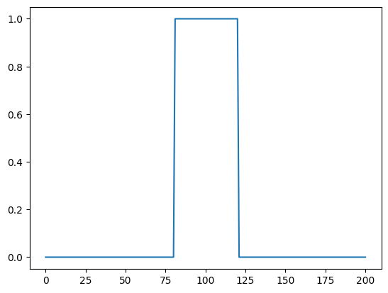
Let us create a function representing a signal that we want to convolve.
signal_function = lambda xi: (xi>np.round(dim*4/10))*(xi<np.round(dim*6/10))
We evaluate the function signal_function at the discretization grid points and wrap it in a CUQIarray object.
signal_array = signal_function(A_deconv.domain_geometry.grid)
signal = CUQIarray(signal_array, geometry=A_deconv.domain_geometry)
Let us plot the signal
signal.plot()
[<matplotlib.lines.Line2D at 0x7f88f8decfd0>]
Now, we evaluate the forward model at the signal and plot the solution:
A_deconv(signal).plot()
[<matplotlib.lines.Line2D at 0x7f88f8c80910>]
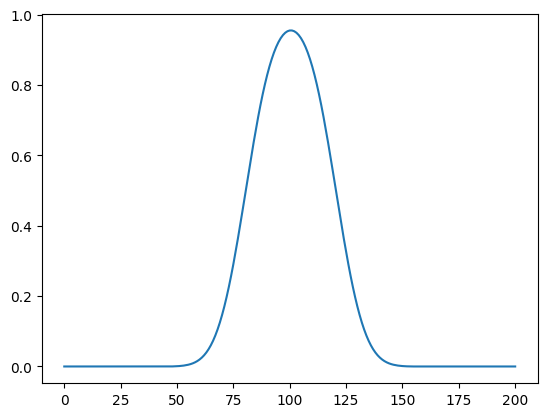
We see that the signal is blurred due to applying the convolution operation (the forward model).
Exercise: #
Type
help(Deconvolution1D)to see the documentation of this test problem.Experimenting with the convolution strength:
Create another convolution model
Bwith the same parameters asA_deconvbut with a differentPSF_paramvalue, usePSF_param=PSF_param/2. Evaluate the forward modelBat the signal and plot the solution along withA_deconv(signal)in the same plot. What do you observe?
Experimenting with setting up the
PSF:Create a new convolution model
Cwith the same parameters asA_deconvbut with a differentPSF, usePSF=np.ones(m)/m. Evaluate the forward modelCat the signal and plot the solution along withA_deconv(signal)in the same plot (try for different values of m: 5, 10, 20). What do you observe?
Experimenting with setting up the
BC:Create a new convolution model
Dwith the same parameters asA_deconvbut with a differentBC, useBC="periodic". Evaluate the forward modelDat the signal and plot the solution along withA_deconv(signal)in the same plot. What do you observe?Now create another signal
another_signalasanother_signal = signal + 0.1*np.exp((D.domain_geometry.grid - np.round(dim*7/8))/10). Plot the new signal. Evaluate the forward modelsA_deconv, andDat the new signal and plot the solutions in the same plot. What do you observe?
Is this true for you: “I can load the pre-existing convolution 1D forward model in CUQIpy, experiment with its parameter setup, evaluate it on some input, and visualize the input and output”? If not, what questions do you have?
# your code here