Two target distributions

Two target distributions#

In this notebook, we define two target distributions:

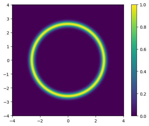
a bi-variate “donut” distribution,
and a posterior distribution for a 1D Poisson-based BIP. that we will use in this chapter to illustrate sampling with CUQIpy. The former target is used for illustrative purposes and is not associated with an inverse problem, while the latter is a more realistic example of a BIP.

We also show high level usage of the BayesianProblem class to explore the posterior distribution as well as defining the target distribution in a more low-level approach through the JointDistribution class.

The “donut” distribution #

In CUQIpy, we provide a set of bi-variate distributions for illustrative purposes. One of these is the “donut” distribution, which is a bi-variate distribution of a donut-shaped. The distribution is defined as follows:

\[ \begin{align}\begin{aligned}\begin{aligned} log (p(\mathbf{x})) \propto - \frac{1}{\sigma_\text{donut}^2} \left( \left\| \mathbf{x} \right\| - r_\text{donut} \right)^2\\\end{aligned}\end{aligned}\end{align} \]

Where \(\mathbf{x} = (x_1, x_2)\) is a 2D vector, \(\left\| \mathbf{x} \right\|\) is the Euclidean norm of \(\mathbf{x}\), \(r_\text{donut}\) is the radius of the donut, and \(\sigma_\text{donut}\) is a scalar value that controls the width of the “donut”.

To load the “donut” distribution, we use the following:

target_donut = DistributionGallery("donut")

print(target_donut)

CUQI DistributionGallery.

We can plot the distribution probability density function (pdf):

plot_pdf_2D(target_donut, -4, 4, -4, 4)

/tmp/ipykernel_1897/3621908757.py:23: DeprecationWarning: Conversion of an array with ndim > 0 to a scalar is deprecated, and will error in future. Ensure you extract a single element from your array before performing this operation. (Deprecated NumPy 1.25.)
  distb_pdf[ii,jj] = np.exp(distb.logd(np.array([grid1[ii,jj], grid2[ii,jj]])))

../_images/6af2725f91a374d0c21172bae84dd5fce31a20b5bb0505e12411807021a154ce.png

A 1D Poisson-based BIP #

The forward model #

Consider a heat conductive rod of length \(L = \pi\) with a varying conductivity (the conductivity of the rod changes from point to point). We fix the temperature at the end-points of the rod and apply a heat source distributed along the length of the rod. We wait until the rod reaches an equilibrium temperature distribution. The equilibrium temperature of the rod is modelled using the second order steady-state PDE as

\[\begin{split} \left\{ \begin{aligned} & \dfrac{\dd}{\dd \xi}\left(u(\xi) \dfrac{\dd y(\xi)}{\dd \xi}\right) = -f(\xi), \quad & \xi\in (0,L) \\ & y(0) = y(L) = 0. \end{aligned} \right. \end{split}\]

Here, \(y\) represents the temperature distribution along the rod, \(u(\xi) \) is the unknown conductivity of the rod and \(f(\xi)\) is a deterministic heat source given by

\[ \begin{aligned} f(\xi) = 10\exp( -\frac{ (\xi - L/2)^2} {0.02} ). \end{aligned} \]

To ensure that the conductivity of the rod is non-negative, we parameterize \(u\) by a random variable \(x\) as follows:

\[ \begin{aligned} u( \cdot ) = \exp( x( \cdot ) ) \end{aligned} \]

where \(x\) is not necessarily positive.

Let us load the forward model that maps the random variable \(x\) to the temperature distribution \(y\) in CUQIpy. We will use the following parameters:

dim : number of discretization points for the rod
L : length of the rod
f : a function that represents the heat source

dim = 201
L = np.pi

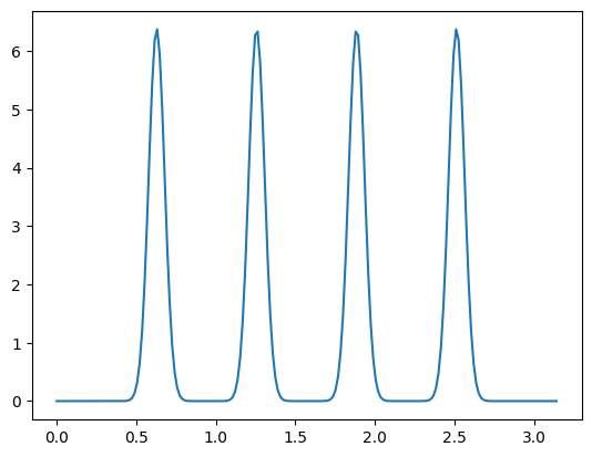
The source term represents spikes at four locations xs with weight ws

xs = np.array([0.2, 0.4, 0.6, 0.8])*L
ws = 0.8
sigma_s = 0.05
def f(t):
    s = np.zeros(dim-1)
    for i in range(4):
        s += ws * sps.norm.pdf(t, loc=xs[i], scale=sigma_s)
    return s

Let us plot the source term for visualization:

temp_grid = np.linspace(0, L, dim-1)
plt.plot(temp_grid, f(temp_grid))

[<matplotlib.lines.Line2D at 0x7fc9089a3160>]

../_images/5f9e307f20bbb087874acde6a091c4e24f94863c703b07e4b838cf8b7fb651d7.png

Then we can load the 1D Poisson forward model as follows:

A, _, _ = Poisson1D(dim=dim, 
                    endpoint=L,
                    field_type='KL',
                    field_params={'num_modes': 10} ,
                    map=lambda x: np.exp(x), 
                    source=f).get_components()

We print the forward model to see its details.

CUQI PDEModel: MappedGeometry(KLExpansion(10,)) -> Continuous1D(200,).
    Forward parameters: ['x'].
    PDE: SteadyStateLinearPDE.

Let us look at the pde property of the forward model:

A.pde

CUQI SteadyStateLinearPDE.
PDE form expression:
        PDE_form = lambda x: (Dx.T @ np.diag(x) @ Dx, rhs)

We can look at the domain and range geometries of the forward model.

print(A.domain_geometry)
print(A.range_geometry)

MappedGeometry(KLExpansion(10,))
Continuous1D(200,)

And inspect the domain geometry further. Let us look at the mapping in the MappedGeometry object.

print(inspect.getsource(A.domain_geometry.map))

                    map=lambda x: np.exp(x),

We can extract the underlying geometry of the MappedGeometry object.

underlying_geometry = A.domain_geometry.geometry
print(underlying_geometry)

KLExpansion(10,)

The underlying geometry represents a Karhunen–Loève (KL) expansion of a random field. Let us look at some of the properties of this underlying_geometry such as the number of modes in the KL expansion and the grid on which the KL expansion basis functions are defined.

print(A.domain_geometry.geometry.num_modes)
print(A.domain_geometry.geometry.grid)

10
[0.         0.01570796 0.03141593 0.04712389 0.06283185 0.07853982
09424778 0.10995574 0.12566371 0.14137167 0.15707963 0.1727876
18849556 0.20420352 0.21991149 0.23561945 0.25132741 0.26703538
28274334 0.2984513  0.31415927 0.32986723 0.34557519 0.36128316
37699112 0.39269908 0.40840704 0.42411501 0.43982297 0.45553093
4712389  0.48694686 0.50265482 0.51836279 0.53407075 0.54977871
56548668 0.58119464 0.5969026  0.61261057 0.62831853 0.64402649
65973446 0.67544242 0.69115038 0.70685835 0.72256631 0.73827427
75398224 0.7696902  0.78539816 0.80110613 0.81681409 0.83252205
84823002 0.86393798 0.87964594 0.89535391 0.91106187 0.92676983
9424778  0.95818576 0.97389372 0.98960169 1.00530965 1.02101761
03672558 1.05243354 1.0681415  1.08384947 1.09955743 1.11526539
13097336 1.14668132 1.16238928 1.17809725 1.19380521 1.20951317
22522113 1.2409291  1.25663706 1.27234502 1.28805299 1.30376095
31946891 1.33517688 1.35088484 1.3665928  1.38230077 1.39800873
41371669 1.42942466 1.44513262 1.46084058 1.47654855 1.49225651
50796447 1.52367244 1.5393804  1.55508836 1.57079633 1.58650429
60221225 1.61792022 1.63362818 1.64933614 1.66504411 1.68075207
69646003 1.712168   1.72787596 1.74358392 1.75929189 1.77499985
79070781 1.80641578 1.82212374 1.8378317  1.85353967 1.86924763
88495559 1.90066356 1.91637152 1.93207948 1.94778745 1.96349541
97920337 1.99491134 2.0106193  2.02632726 2.04203522 2.05774319
07345115 2.08915911 2.10486708 2.12057504 2.136283   2.15199097
16769893 2.18340689 2.19911486 2.21482282 2.23053078 2.24623875
26194671 2.27765467 2.29336264 2.3090706  2.32477856 2.34048653
35619449 2.37190245 2.38761042 2.40331838 2.41902634 2.43473431
45044227 2.46615023 2.4818582  2.49756616 2.51327412 2.52898209
54469005 2.56039801 2.57610598 2.59181394 2.6075219  2.62322987
63893783 2.65464579 2.67035376 2.68606172 2.70176968 2.71747765
73318561 2.74889357 2.76460154 2.7803095  2.79601746 2.81172542
82743339 2.84314135 2.85884931 2.87455728 2.89026524 2.9059732
92168117 2.93738913 2.95309709 2.96880506 2.98451302 3.00022098
01592895 3.03163691 3.04734487 3.06305284 3.0787608  3.09446876
11017673 3.12588469 3.14159265]

The range geometry is of type Continuous1D which represents a 1D continuous signal/field defined on a grid. We can view the grid:

print(A.domain_geometry.grid)

[0.         0.01570796 0.03141593 0.04712389 0.06283185 0.07853982
09424778 0.10995574 0.12566371 0.14137167 0.15707963 0.1727876
18849556 0.20420352 0.21991149 0.23561945 0.25132741 0.26703538
28274334 0.2984513  0.31415927 0.32986723 0.34557519 0.36128316
37699112 0.39269908 0.40840704 0.42411501 0.43982297 0.45553093
4712389  0.48694686 0.50265482 0.51836279 0.53407075 0.54977871
56548668 0.58119464 0.5969026  0.61261057 0.62831853 0.64402649
65973446 0.67544242 0.69115038 0.70685835 0.72256631 0.73827427
75398224 0.7696902  0.78539816 0.80110613 0.81681409 0.83252205
84823002 0.86393798 0.87964594 0.89535391 0.91106187 0.92676983
9424778  0.95818576 0.97389372 0.98960169 1.00530965 1.02101761
03672558 1.05243354 1.0681415  1.08384947 1.09955743 1.11526539
13097336 1.14668132 1.16238928 1.17809725 1.19380521 1.20951317
22522113 1.2409291  1.25663706 1.27234502 1.28805299 1.30376095
31946891 1.33517688 1.35088484 1.3665928  1.38230077 1.39800873
41371669 1.42942466 1.44513262 1.46084058 1.47654855 1.49225651
50796447 1.52367244 1.5393804  1.55508836 1.57079633 1.58650429
60221225 1.61792022 1.63362818 1.64933614 1.66504411 1.68075207
69646003 1.712168   1.72787596 1.74358392 1.75929189 1.77499985
79070781 1.80641578 1.82212374 1.8378317  1.85353967 1.86924763
88495559 1.90066356 1.91637152 1.93207948 1.94778745 1.96349541
97920337 1.99491134 2.0106193  2.02632726 2.04203522 2.05774319
07345115 2.08915911 2.10486708 2.12057504 2.136283   2.15199097
16769893 2.18340689 2.19911486 2.21482282 2.23053078 2.24623875
26194671 2.27765467 2.29336264 2.3090706  2.32477856 2.34048653
35619449 2.37190245 2.38761042 2.40331838 2.41902634 2.43473431
45044227 2.46615023 2.4818582  2.49756616 2.51327412 2.52898209
54469005 2.56039801 2.57610598 2.59181394 2.6075219  2.62322987
63893783 2.65464579 2.67035376 2.68606172 2.70176968 2.71747765
73318561 2.74889357 2.76460154 2.7803095  2.79601746 2.81172542
82743339 2.84314135 2.85884931 2.87455728 2.89026524 2.9059732
92168117 2.93738913 2.95309709 2.96880506 2.98451302 3.00022098
01592895 3.03163691 3.04734487 3.06305284 3.0787608  3.09446876
11017673 3.12588469 3.14159265]

Additionally, the properties domain_dim and range_dim of the forward model represent the dimension of the input and output of the forward model, respectively.

print(A.domain_dim)
print(A.range_dim)

10
200

The BIP: the prior #

We now build a posterior distribution based on this forward model. The unknown \(\mathbf{x}\) represents the coefficients in the KL expansion. We assume that the prior distribution of \(\mathbf{x}\) is an i.i.d Gaussian distribution with mean \(0\) and variance \(\sigma_x^2\).

sigma_x = 30
x = Gaussian(0, sigma_x**2, geometry=A.domain_geometry)

Let us assume that the true solution we want to infer is a sample from x. Note: we fix the random seed for reproducibility.

np.random.seed(12)
x_true = x.sample()

Exercise #

Visualize x_true in the KL coefficient space. Hint: try x_true.plot(plot_par=True)
Visualize x_true in the corresponding function space (after applying the linear combination of KL basis weighted by KL vectors and then applying the exponantial mapping). Hint: all this can be achieved in one line by x_true.plot(plot_par=False)

# your code here

The BIP: the likelihood #

We assume the data we obtain is a noisy measurement of the temperature \(y\) over the interval \([0, L]\) in all grid points. The measurements form a vector \(\mathbf{y}\). The noise is assumed to be additive Gaussian noise with mean \(0\) and variance \(\sigma_y^2\).

\[ \mathbf{y} = \mathbf{A}(\mathbf{x}) + \epsilon \quad \text{where} \quad \epsilon \sim \mathcal{N}(0, \sigma_y^2).\]

We define the data distribution \(p(\mathbf{y} | \mathbf{x})\) in CUQIpy in this case as

sigma_y = np.sqrt(0.001)
y = Gaussian(A(x), sigma_y**2, geometry=A.range_geometry)

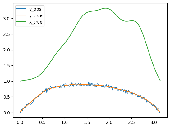
We create a synthetic data to use it to test solving our BIP. We denote this data as \(\mathbf{y}_{\text{obs}}\) which is a particular observed data realization from a setup where the KL coefficients are x_true. To create this data in CUQIpy, we use the following:

y_obs = y(x=x_true).sample()

Let us plot the true conductivity field, corresponding to x_true, the data y_true without noise i.e. A(x_true), and the noisy data y_obs in the same plot.

y_obs.plot(label='y_obs')
A(x_true).plot(label='y_true')
x_true.plot(label='x_true')
plt.legend()

<matplotlib.legend.Legend at 0x7fc9058171c0>

../_images/30fd50e7d2596f2eb4c602459ed09cb52a56f27c234b6733025078aa859cb35d.png

The BIP: the posterior distribution (the high level approach: using the BayesianProblem class)#

The posterior distribution of the Bayesian inverse problem in this case is given by

\[ \begin{align*} p(\mathbf{x} \mid \mathbf{y}=\mathbf{y}_\mathrm{obs}) \propto L(\mathbf{x} \mid \mathbf{y}=\mathbf{y}_\mathrm{obs})p(\mathbf{x}), \end{align*} \]

where we use the notation \(L(\mathbf{x} \mid \mathbf{y}=\mathbf{y}_\mathrm{obs}) := p(\mathbf{y}=\mathbf{y}_\mathrm{obs} \mid \mathbf{x})\) for the likelihood function to emphasize that, in the context of the posterior where \(\mathbf{y}\) is fixed to \(\mathbf{y}_\mathrm{obs}\), it is a function of \(\mathbf{x}\) and not on \(\mathbf{y}\). In CUQIpy we sometimes use the short-hand printing style L(x|y) for brevity.

The simplest way to sample a Bayesian inverse problem in CUQIpy is to use the BayesianProblem class.

Using the BayesianProblem class, one can easily define and sample from the posterior distribution of a Bayesian inverse problem by providing the distributions for the parameters and data and subsequently setting the observed data.

BP_poisson = BayesianProblem(x, y)      # Create Bayesian problem
BP_poisson.set_data(y=y_obs)           # Provide observed data

BayesianProblem with target: 
 Posterior(
    Equation:
	 p(x|y) ∝ L(x|y)p(x)
    Densities:
	y ~ CUQI Gaussian Likelihood function. Parameters ['x'].
 	x ~ CUQI Gaussian.
 )

In the above example, we provided our assumptions about the data generating process by defining the distributions for the parameters and data and provided the observed data for the problem. CUQIpy internally created the posterior distribution using the provided distributions and data.

We can use this object to sample from the posterior distribution using the UQ method, which we will experiment with in this exercise:

Exercise #

Use the UQ method of the BP_poisson object to sample the posterior distribution. The UQ returns a Samples object, store the result in a variable called BP_poisson_samples.

# your code here

In the previous exercise we saw that CUQIpy automatically decided on using a sampler, preconditioned Crank Nicolson pCN in this case, and sampled the posterior distribution. Additionally, the credibility interval for the parameter \(\mathbf{x}\) as well as the mean of the posterior was plotted and compared to the ground truth (x_true).

Note about visualizing the credible interval: Using the UQ method, the credibility interval is computed for the KL coefficients. Then mapped to the function space and plotted. We can also compute the credibility interval directly on the function values. We will revisit this at a later stage.

In the next section, we show how to define the posterior distribution more explicitly.

The BIP: computing the MAP point with the BayesianProblem class#

In addition to sampling the posterior, we can also compute point estimates of the posterior. A common point estimate to consider is the Maximum A Posteriori (MAP) estimate, which is the value of the Bayesian parameter that maximizes the posterior density. That is,

\[ \begin{align*} \mathbf{x}_\mathrm{MAP} = \arg\max_\mathbf{x} p(\mathbf{x} \mid \mathbf{y}_\mathrm{obs}). \end{align*} \]

The easiest way to compute the MAP estimate in CUQIpy is to use the MAP method of the BayesianProblem class as follows:

# x_map = BP_poisson.MAP()

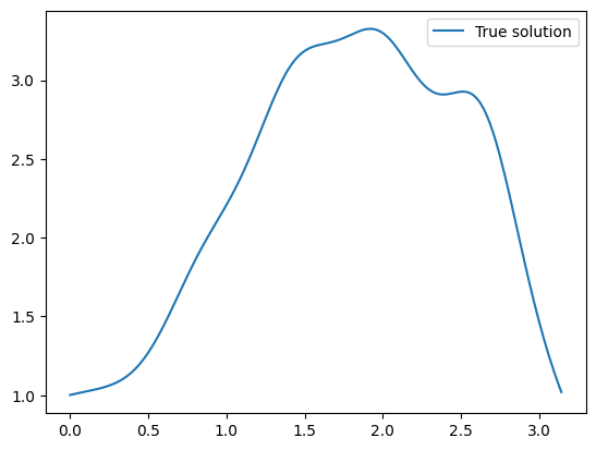
We can plot the MAP estimate and compare it to the true solution x_true.

# x_map.plot(label='MAP estimate')
x_true.plot(label='True solution')
plt.legend()

<matplotlib.legend.Legend at 0x7fc950b5d8a0>

../_images/20be41985349b182e9f1814a83b0b15bf3222e5aa981cbcfe147c7ea95842a20.png

We can also look at the MAP estimate in the KL coefficient space:

# x_map.plot(label='MAP estimate' ,plot_par=True)
x_true.plot(label='True solution' ,plot_par=True)
plt.legend()

<matplotlib.legend.Legend at 0x7fc9058c30a0>

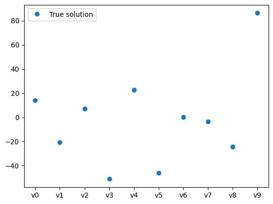
../_images/73e9fe6b4f82a1a27c677afbe04a46cb73d93305c7f4f509c41a351becf3175b.png

We notice that in general the larger the mode number, the harder it is to be inferred (can you think why?).

The BIP: the posterior distribution (the low level approach: using the JointDistribution)#

To define the posterior distribution explicitly in CUQIpy, we first define the joint distribution \(p(\mathbf{y},\mathbf{x})\), then we supply the observed data to create the conditional distribution \(p(\mathbf{x} \mid \mathbf{y}=\mathbf{y}_\mathrm{obs})\).

Let us first define the joint distribution \(p(\mathbf{y},\mathbf{x})\) in CUQIpy. We use the following:

# Define joint distribution p(y,x)
joint = JointDistribution(y, x)

Calling print on the joint distribution gives a nice overview matching the mathematical description of the joint distribution.

print(joint)

JointDistribution(
    Equation: 
	p(y,x) = p(y|x)p(x)
    Densities: 
	y ~ CUQI Gaussian. Conditioning variables ['x'].
	x ~ CUQI Gaussian.
)

CUQIpy can automatically derive the posterior distribution for any joint distribution when we pass the observed data as an argument to the “call” (condition) method of the joint distribution. This is done as follows:

target_poisson = joint(y=y_obs) # Condition p(x,y) on y=y_data. Applies Bayes' rule automatically

We can now inspect the posterior distribution by calling print on it. Notice that the posterior equation matches the mathematical expression we showed above.

print(target_poisson)

Posterior(
    Equation:
	 p(x|y) ∝ L(x|y)p(x)
    Densities:
	y ~ CUQI Gaussian Likelihood function. Parameters ['x'].
 	x ~ CUQI Gaussian.
 )

Exercise #

The posterior is essentially just another CUQIpy distribution. Have a look at the Posterior class in the online documentation to see what attributes and methods are available.
Try evaluating the posterior log probability density function (logpdf) and pdf at some points say x_true and x_true*1.1.

# Your code here

Two target distributions

Contents

Two target distributions#

The “donut” distribution #

A 1D Poisson-based BIP #

The forward model #

The BIP: the prior #

Exercise #

The BIP: the likelihood #

The BIP: the posterior distribution (the high level approach: using the BayesianProblem class)#

Exercise #

The BIP: computing the MAP point with the BayesianProblem class#

The BIP: the posterior distribution (the low level approach: using the JointDistribution)#

Exercise #