Note
Go to the end to download the full example code.
Setting a Bayesian model with multiple likelihoods#
In this example we build a PDE-based Bayesian inverse problem where the Bayesian
model has multiple likelihood functions (two different likelihood functions in
this case, but it can be readily extended to more functions) for the same
Bayesian parameter theta, which represents the conductivity parameters in a
1D Poisson problem. Each likelihood is associated with a different model set
up. The models we use here are obtained from the test problem
cuqi.testproblem.Poisson1D. See the class
cuqi.testproblem.Poisson1D documentation for more details about the
forward model.
First we import the python libraries needed.
import cuqi
import numpy as np
import matplotlib.pyplot as plt
from math import ceil
Choose one of the two cases we study in this demo#
We can choose between two cases: Choose set_up = set_ups[0] for the case where we have two 1D Poisson models that differ in the observation operator only. And choose set_up = set_ups[1] for the case where we have two 1D Poisson models that differ in the source term only. Here we demonstrate the first case, set_up = set_ups[0].
set_ups = ["multi_observation", "multi_source"]
set_up = set_ups[0]

assert set_up == "multi_observation" or set_up == "multi_source",\
    "set_up must be either 'multi_observation' or 'multi_source'"
Set up the parameters used in both models#
dim = 50  # Number of the model grid points
endpoint = 1  # The model domain is the interval [0, endpoint]
field_type = "Step"  # The conductivity (or diffusivity) field type.
                     # We choose step function parameterization here.
SNR = 400  # Signal-to-noise ratio
n_steps = 2  # Number of steps in the conductivity (or diffusivity) step field
magnitude = 100 # Magnitude of the source term in the Poisson problem

# Exact solution
x_exact = np.empty(dim)
x_exact[:ceil(dim/2)] = 2
x_exact[ceil(dim/2):] = 3
Set up the first model#
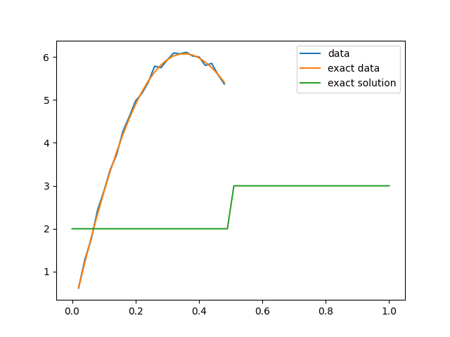
We set up the first forward model to have observations at the first half of the domain (or observation everywhere if set_up = set_ups[1]). We then plot the true conductivity field (the exact solution), the exact data and the noisy data.
observation_grid_map1 = None
if set_up == "multi_observation":
    # Observe on the first half of the domain
    observation_grid_map1 = lambda x: x[np.where(x<.5)]

# The source term signal
source1 = lambda xs: magnitude*np.sin(xs*2*np.pi/endpoint)+magnitude

# Obtain the forward model from the test problem
model1, data1, problemInfo1 = cuqi.testproblem.Poisson1D(dim=dim,
    endpoint=endpoint,
    field_type=field_type,
    field_params={"n_steps": n_steps},
    observation_grid_map=observation_grid_map1,
    exactSolution=x_exact,
    source=source1,
    SNR=SNR).get_components()

# Plot data, exact data and exact solution
plt.figure()
data1.plot(label='data')
problemInfo1.exactData.plot(label='exact data')
problemInfo1.exactSolution.plot(label='exact solution')
plt.legend()
<matplotlib.legend.Legend object at 0x7f18aade11c0>
Set up the second model#
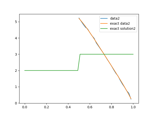
We set up the second forward model to have observations at the second half of the domain (or observation everywhere and and different source term if set_up = set_ups[1]). We then plot the true conductivity field (the exact solution), the exact data and the noisy data.
observation_grid_map2 = None
if set_up == "multi_observation":
        # Observe on the second half of the domain
    observation_grid_map2 = lambda x: x[np.where(x>=.5)]

# The source term signal
if set_up == "multi_source":
    source2 = lambda xs: magnitude*np.sin(2*xs*2*np.pi/endpoint)+magnitude
else:
    source2 = source1

# Obtain the forward model from the test problem
model2, data2, problemInfo2 = cuqi.testproblem.Poisson1D(dim=dim,
    endpoint=endpoint,
    field_type=field_type,
    field_params={"n_steps": n_steps},
    observation_grid_map=observation_grid_map2,
    exactSolution=x_exact,
    source=source2,
    SNR=SNR).get_components()

# Plot data, exact data and exact solution
plt.figure()
data2.plot(label='data2')
problemInfo2.exactData.plot(label='exact data2')
problemInfo2.exactSolution.plot(label='exact solution2')
plt.legend()
<matplotlib.legend.Legend object at 0x7f1891782cf0>
Create the prior#
Create the prior for the Bayesian parameter theta, which is the expansion coefficients of the conductivity (or diffusivity) step function. We use a Gaussian prior.
theta = cuqi.distribution.Gaussian(
    mean=np.zeros(model1.domain_dim),
    cov=3,
    geometry=model1.domain_geometry,
)
Create the data distributions using the two forward models#
# Estimate the data noise standard deviation
sigma_noise1 = np.linalg.norm(problemInfo1.exactData)/SNR
sigma_noise2 = np.linalg.norm(problemInfo2.exactData)/SNR

# Create the data distributions
y1 = cuqi.distribution.Gaussian(
    mean=model1(theta),
    cov=sigma_noise1**2,
    geometry=model1.range_geometry,
)
y2 = cuqi.distribution.Gaussian(
    mean=model2(theta),
    cov=sigma_noise2**2,
    geometry=model2.range_geometry,
)
Formulate the Bayesian inverse problem using the first data distribution (single likelihood)#
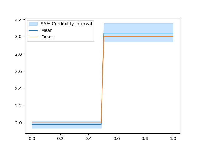
We first formulate the Bayesian inverse problem using the first data distribution and analyze the posterior samples.
Create the posterior#
z1 = cuqi.distribution.JointDistribution(theta,y1)(y1=data1)
We print the joint distribution z1:
print(z1)
Posterior(
    Equation:
         p(theta|y1) ∝ L(theta|y1)p(theta)
    Densities:
        y1 ~ CUQI Gaussian Likelihood function. Parameters ['theta'].
        theta ~ CUQI Gaussian.
 )
We see that we obtain a cuqi.distribution.Posterior object, which
represents the posterior distribution of the parameters theta given the data
y1. The posterior distribution in this case is proportional to the product
of the likelihood obtained from the first data distribution and the prior.
Sample from the posterior#
# Sample from the posterior
sampler = cuqi.legacy.sampler.MH(z1)
samples = sampler.sample_adapt(8000)

# Plot the credible interval and compute the ESS
samples.burnthin(1000).plot_ci(95, exact=problemInfo1.exactSolution)
samples.compute_ess()
/home/runner/work/CUQIpy/CUQIpy/cuqi/legacy/sampler/_sampler.py:156: UserWarning:
You are using the legacy sampler 'MH'.
This will be removed in a future release of CUQIpy.
Please consider using the new samplers in the 'cuqi.sampler' module.

  super().__init__(target, x0=x0, dim=dim, **kwargs)

Sample 80 / 8000
Sample 160 / 8000
Sample 240 / 8000
Sample 320 / 8000
Sample 400 / 8000
Sample 480 / 8000
Sample 560 / 8000
Sample 640 / 8000
Sample 720 / 8000
Sample 800 / 8000
Sample 880 / 8000
Sample 960 / 8000
Sample 1040 / 8000
Sample 1120 / 8000
Sample 1200 / 8000
Sample 1280 / 8000
Sample 1360 / 8000
Sample 1440 / 8000
Sample 1520 / 8000
Sample 1600 / 8000
Sample 1680 / 8000
Sample 1760 / 8000
Sample 1840 / 8000
Sample 1920 / 8000
Sample 2000 / 8000
Sample 2080 / 8000
Sample 2160 / 8000
Sample 2240 / 8000
Sample 2320 / 8000
Sample 2400 / 8000
Sample 2480 / 8000
Sample 2560 / 8000
Sample 2640 / 8000
Sample 2720 / 8000
Sample 2800 / 8000
Sample 2880 / 8000
Sample 2960 / 8000
Sample 3040 / 8000
Sample 3120 / 8000
Sample 3200 / 8000
Sample 3280 / 8000
Sample 3360 / 8000
Sample 3440 / 8000
Sample 3520 / 8000
Sample 3600 / 8000
Sample 3680 / 8000
Sample 3760 / 8000
Sample 3840 / 8000
Sample 3920 / 8000
Sample 4000 / 8000
Sample 4080 / 8000
Sample 4160 / 8000
Sample 4240 / 8000
Sample 4320 / 8000
Sample 4400 / 8000
Sample 4480 / 8000
Sample 4560 / 8000
Sample 4640 / 8000
Sample 4720 / 8000
Sample 4800 / 8000
Sample 4880 / 8000
Sample 4960 / 8000
Sample 5040 / 8000
Sample 5120 / 8000
Sample 5200 / 8000
Sample 5280 / 8000
Sample 5360 / 8000
Sample 5440 / 8000
Sample 5520 / 8000
Sample 5600 / 8000
Sample 5680 / 8000
Sample 5760 / 8000
Sample 5840 / 8000
Sample 5920 / 8000
Sample 6000 / 8000
Sample 6080 / 8000
Sample 6160 / 8000
Sample 6240 / 8000
Sample 6320 / 8000
Sample 6400 / 8000
Sample 6480 / 8000
Sample 6560 / 8000
Sample 6640 / 8000
Sample 6720 / 8000
Sample 6800 / 8000
Sample 6880 / 8000
Sample 6960 / 8000
Sample 7040 / 8000
Sample 7120 / 8000
Sample 7200 / 8000
Sample 7280 / 8000
Sample 7360 / 8000
Sample 7440 / 8000
Sample 7520 / 8000
Sample 7600 / 8000
Sample 7680 / 8000
Sample 7760 / 8000
Sample 7840 / 8000
Sample 7920 / 8000
Sample 8000 / 8000
Sample 8000 / 8000

Average acceptance rate: 0.10475 MCMC scale: 0.05223526807427086


array([274.54145793, 192.80680791])
Formulate the Bayesian inverse problem using the second data distribution (single likelihood)#
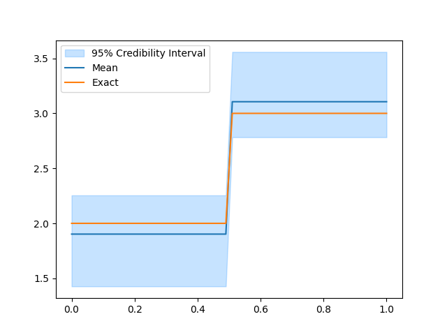
We then formulate the Bayesian inverse problem using the second data distribution and analyze the posterior samples.
Create the posterior#
z2 = cuqi.distribution.JointDistribution(theta,y2)(y2=data2)
We print the joint distribution z2:
print(z2)
Posterior(
    Equation:
         p(theta|y2) ∝ L(theta|y2)p(theta)
    Densities:
        y2 ~ CUQI Gaussian Likelihood function. Parameters ['theta'].
        theta ~ CUQI Gaussian.
 )
We see that we obtain a cuqi.distribution.Posterior object, which
represents the posterior distribution of the parameters theta given the data
y2. The posterior distribution in this case is proportional to the product
of the likelihood obtained from the second data distribution and the prior.
Sample from the posterior#
# Sample from the posterior
sampler = cuqi.legacy.sampler.MH(z2)
samples = sampler.sample_adapt(8000)

# Plot the credible interval and compute the ESS
samples.burnthin(1000).plot_ci(95, exact=problemInfo1.exactSolution)
samples.compute_ess()
/home/runner/work/CUQIpy/CUQIpy/cuqi/legacy/sampler/_sampler.py:156: UserWarning:
You are using the legacy sampler 'MH'.
This will be removed in a future release of CUQIpy.
Please consider using the new samplers in the 'cuqi.sampler' module.

  super().__init__(target, x0=x0, dim=dim, **kwargs)

Sample 80 / 8000
Sample 160 / 8000
Sample 240 / 8000
Sample 320 / 8000
Sample 400 / 8000
Sample 480 / 8000
Sample 560 / 8000
Sample 640 / 8000
Sample 720 / 8000
Sample 800 / 8000
Sample 880 / 8000
Sample 960 / 8000
Sample 1040 / 8000
Sample 1120 / 8000
Sample 1200 / 8000
Sample 1280 / 8000
Sample 1360 / 8000
Sample 1440 / 8000
Sample 1520 / 8000
Sample 1600 / 8000
Sample 1680 / 8000
Sample 1760 / 8000
Sample 1840 / 8000
Sample 1920 / 8000
Sample 2000 / 8000
Sample 2080 / 8000
Sample 2160 / 8000
Sample 2240 / 8000
Sample 2320 / 8000
Sample 2400 / 8000
Sample 2480 / 8000
Sample 2560 / 8000
Sample 2640 / 8000
Sample 2720 / 8000
Sample 2800 / 8000
Sample 2880 / 8000
Sample 2960 / 8000
Sample 3040 / 8000
Sample 3120 / 8000
Sample 3200 / 8000
Sample 3280 / 8000
Sample 3360 / 8000
Sample 3440 / 8000
Sample 3520 / 8000
Sample 3600 / 8000
Sample 3680 / 8000
Sample 3760 / 8000
Sample 3840 / 8000
Sample 3920 / 8000
Sample 4000 / 8000
Sample 4080 / 8000
Sample 4160 / 8000
Sample 4240 / 8000
Sample 4320 / 8000
Sample 4400 / 8000
Sample 4480 / 8000
Sample 4560 / 8000
Sample 4640 / 8000
Sample 4720 / 8000
Sample 4800 / 8000
Sample 4880 / 8000
Sample 4960 / 8000
Sample 5040 / 8000
Sample 5120 / 8000
Sample 5200 / 8000
Sample 5280 / 8000
Sample 5360 / 8000
Sample 5440 / 8000
Sample 5520 / 8000
Sample 5600 / 8000
Sample 5680 / 8000
Sample 5760 / 8000
Sample 5840 / 8000
Sample 5920 / 8000
Sample 6000 / 8000
Sample 6080 / 8000
Sample 6160 / 8000
Sample 6240 / 8000
Sample 6320 / 8000
Sample 6400 / 8000
Sample 6480 / 8000
Sample 6560 / 8000
Sample 6640 / 8000
Sample 6720 / 8000
Sample 6800 / 8000
Sample 6880 / 8000
Sample 6960 / 8000
Sample 7040 / 8000
Sample 7120 / 8000
Sample 7200 / 8000
Sample 7280 / 8000
Sample 7360 / 8000
Sample 7440 / 8000
Sample 7520 / 8000
Sample 7600 / 8000
Sample 7680 / 8000
Sample 7760 / 8000
Sample 7840 / 8000
Sample 7920 / 8000
Sample 8000 / 8000
Sample 8000 / 8000

Average acceptance rate: 0.147375 MCMC scale: 0.06429969523036719


array([15.98082264, 15.66716395])
Formulate the Bayesian inverse problem using both data distributions (multiple likelihoods)#
We then formulate the Bayesian inverse problem using both data distributions and analyze the posterior samples.
Create the posterior#
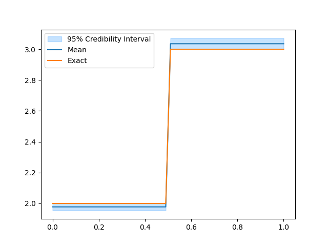
z_joint = cuqi.distribution.JointDistribution(theta,y1,y2)(y1=data1, y2=data2)
We print the joint distribution z_joint:
print(z_joint)
MultipleLikelihoodPosterior(
    Equation:
        p(theta|y1,y2) ∝ p(theta)L(theta|y1)L(theta|y2)
    Densities:
        theta ~ CUQI Gaussian.
        y1 ~ CUQI Gaussian Likelihood function. Parameters ['theta'].
        y2 ~ CUQI Gaussian Likelihood function. Parameters ['theta'].
 )
We see that in this case we obtain a MultipleLikelihoodPosterior
object, which represents the posterior distribution of the parameters theta
given the data y1 and y2. The posterior distribution in this case is
proportional to the product of the two likelihoods and the prior.
Sample from the posterior#
# Sample from the posterior
sampler = cuqi.legacy.sampler.MH(z_joint)
samples = sampler.sample_adapt(8000)

# Plot the credible interval and compute the ESS
samples.burnthin(1000).plot_ci(95, exact=problemInfo1.exactSolution)
samples.compute_ess()
/home/runner/work/CUQIpy/CUQIpy/cuqi/legacy/sampler/_sampler.py:156: UserWarning:
You are using the legacy sampler 'MH'.
This will be removed in a future release of CUQIpy.
Please consider using the new samplers in the 'cuqi.sampler' module.

  super().__init__(target, x0=x0, dim=dim, **kwargs)

Sample 80 / 8000
Sample 160 / 8000
Sample 240 / 8000
Sample 320 / 8000
Sample 400 / 8000
Sample 480 / 8000
Sample 560 / 8000
Sample 640 / 8000
Sample 720 / 8000
Sample 800 / 8000
Sample 880 / 8000
Sample 960 / 8000
Sample 1040 / 8000
Sample 1120 / 8000
Sample 1200 / 8000
Sample 1280 / 8000
Sample 1360 / 8000
Sample 1440 / 8000
Sample 1520 / 8000
Sample 1600 / 8000
Sample 1680 / 8000
Sample 1760 / 8000
Sample 1840 / 8000
Sample 1920 / 8000
Sample 2000 / 8000
Sample 2080 / 8000
Sample 2160 / 8000
Sample 2240 / 8000
Sample 2320 / 8000
Sample 2400 / 8000
Sample 2480 / 8000
Sample 2560 / 8000
Sample 2640 / 8000
Sample 2720 / 8000
Sample 2800 / 8000
Sample 2880 / 8000
Sample 2960 / 8000
Sample 3040 / 8000
Sample 3120 / 8000
Sample 3200 / 8000
Sample 3280 / 8000
Sample 3360 / 8000
Sample 3440 / 8000
Sample 3520 / 8000
Sample 3600 / 8000
Sample 3680 / 8000
Sample 3760 / 8000
Sample 3840 / 8000
Sample 3920 / 8000
Sample 4000 / 8000
Sample 4080 / 8000
Sample 4160 / 8000
Sample 4240 / 8000
Sample 4320 / 8000
Sample 4400 / 8000
Sample 4480 / 8000
Sample 4560 / 8000
Sample 4640 / 8000
Sample 4720 / 8000
Sample 4800 / 8000
Sample 4880 / 8000
Sample 4960 / 8000
Sample 5040 / 8000
Sample 5120 / 8000
Sample 5200 / 8000
Sample 5280 / 8000
Sample 5360 / 8000
Sample 5440 / 8000
Sample 5520 / 8000
Sample 5600 / 8000
Sample 5680 / 8000
Sample 5760 / 8000
Sample 5840 / 8000
Sample 5920 / 8000
Sample 6000 / 8000
Sample 6080 / 8000
Sample 6160 / 8000
Sample 6240 / 8000
Sample 6320 / 8000
Sample 6400 / 8000
Sample 6480 / 8000
Sample 6560 / 8000
Sample 6640 / 8000
Sample 6720 / 8000
Sample 6800 / 8000
Sample 6880 / 8000
Sample 6960 / 8000
Sample 7040 / 8000
Sample 7120 / 8000
Sample 7200 / 8000
Sample 7280 / 8000
Sample 7360 / 8000
Sample 7440 / 8000
Sample 7520 / 8000
Sample 7600 / 8000
Sample 7680 / 8000
Sample 7760 / 8000
Sample 7840 / 8000
Sample 7920 / 8000
Sample 8000 / 8000
Sample 8000 / 8000

Average acceptance rate: 0.066 MCMC scale: 0.04433673360133622


array([216.80214526, 167.15407891])
We notice that combining the two data distributions leads to a more certain estimate of the conductivity (using the same number of MCMC iterations). This is because including the two different data sets in the inversion is more informative than the single data set case. Also, the effective sample size is larger than (or comparable to) what is obtained in any of the single data distribution case.
Total running time of the script: (0 minutes 18.731 seconds)
