Here we dive into forward models in CUQIpy. In brief, a forward model is defined as a mathematical model that describes the relationship between some input parameters (which are not directly observable) and some output data (which is observable). As an example, in image deblurring, the forward model is a mathematical model of the blurring that maps a sharp unknown image to the observed blurred image.
In the context of inverse problems, forward models are an important concept. The forward model can be insensitive to certain changes in the input parameters, which means that different input parameters can produce similar output data. This insensitivity can make it difficult to recover the input parameters from the output data, and inverse problems are therefore often ill-posed. In general, an inverse problem is considered ill-posed if the existence, uniqueness and/or stability of the inversion cannot be guaranteed. This ill-posedness deserves a separate discussion, which is beyond the scope of this section and we refer to Hansen (2010) for the interested reader.
For the purpose of this notebook, we show the basics of how to use forward models in CUQIpy. In particular for generating simulated noisy data and some forward uncertainty quantification. Finally, we also show how to define new custom linear or non-linear forward models in CUQIpy from either a matrix or functions.
Table of contents
1.1. Learning objectives
1.2. Access forward models from test problems
1.3. Basic usage of forward models
1.4. Generating synthetic data
1.5. Creating custom forward models
1.1. Learning objectives 
Going through this notebook you will see how to
Access and use pre-defined forward models from the CUQIpy
testproblemlibrary.Carry out basic operations of forward models such as forward evaluation.
Generate noisy forward simulated data.
Make a custom forward model from an existing matrix or function.
★ Indicates optional sections and exercises.
Before getting started, we have to import the Python packages we need. Here we also import CUQIpy (cuqi).
import numpy as np
import matplotlib.pyplot as plt
import cuqi
np.random.seed(0)
1.2. Access forward models from test problems
Forward models in CUQIpy are the link between the parameter of interest (which we call solution), say , and the observed data, say . In their simplest form, they are simply a mapping , which we refer to as the forward map. In CUQIpy, forward models are so commonly used that we refer to them simply as models.
In addition to providing a mapping for the “forward” operation and potentially the adjoint, a CUQIpy model also contains information on the parametrization and potentially the discretization of its domain and range, as well as available gradients and so on.
To get a better grasp of the extend of CUQIpy models, let us look at a few examples taken from CUQIpy’s testproblem library.
A CUQIpy test problem contains all components specifying an inverse problem, including example data. Most test problems can be configured in different ways. A simple way to work with test problems is to return the main components, namely the forward model, the data and dictionary with problem information.
1.2.1. Deconvolution in 1D
For example, we can set up a 1D Deconvolution test problem and return the main components by:
testproblem1 = cuqi.testproblem.Deconvolution1D(dim=64, phantom="sinc")
model1, data1, probInfo1 = testproblem1.get_components()
We define testproblem1 with mostly default settings, except for the dimension and type of phantom. Here we mean by phantom the true image or signal we want to recover from the data.
Calling print around the model gives us some of the most important information about the model:
print(model1)CUQI LinearModel: Continuous1D[64] -> Continuous1D[64].
Forward parameters: ['x'].
In this case, we see that we are working with a LinearModel (linear in the operator sense), which makes sense for the deconvolution problem. We also see that the domain and range are both parametrized as Continous1D with 64 parameters. Finally, we see that the forward parameter is called ‘x’.
The problem info typically contains both the exact synthetic signal exactSolution from which the data was produced and the exact simulated data exactData:
probInfo1ProblemInfo with the following set attributes:
['exactSolution', 'exactData', 'infoString']
infoString: Noise type: Additive Gaussian with std: 0.01The true signal (before blurring) looks like this:
probInfo1.exactSolution.plot()
plt.title("Exact Solution");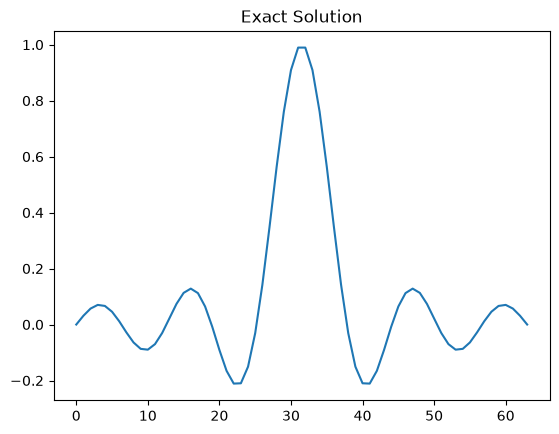
We can plot and compare the clean and noisy data:
data1.plot(label='Noisy data')
probInfo1.exactData.plot(label='Exact data')
plt.legend()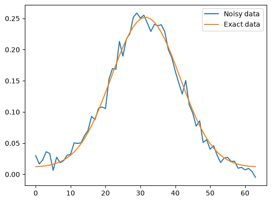
and easily take a look also at their difference, which is the added synthetic noise:
(data1-probInfo1.exactData).plot()
plt.title("Noise realization");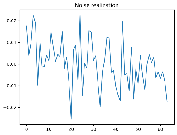
1.2.2. Deconvolution2D: Inverse problem of two-dimensional image deblurring
CUQIpy offers a 2D image deblurring test problem as well, which can be set up in the same way as the 1D problem (now with all default settings):
testproblem2 = cuqi.testproblem.Deconvolution2D()
model2, data2, probInfo2 = testproblem2.get_components()
If we take a look at the model, we see it is a linear model, now with a predetermined Image2D geometries instead of Continuous1D as before - the size corresponds to image of size 128x128 = 16384 pixels:
model2CUQI LinearModel: Image2D[16384: (128, 128)] -> Image2D[16384: (128, 128)].
Forward parameters: ['x'].The Image2D geometries were specified to provide a representation of the model input and output, 2D images. The exact solution is available and plot method displays it as an image due to the predetermined Image2D geometry:
probInfo2.exactSolution.plot()
plt.title("Exact Solution (sharp image)");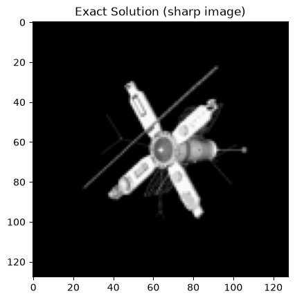
Similarly the blurred and noisy data, the clean data and their difference (i.e. the added noise) can be displayed as images:
data2.plot()
plt.title("Data (noisy blurred image)");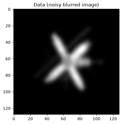
probInfo2.exactData.plot()
plt.title("Exact data (blurred image)");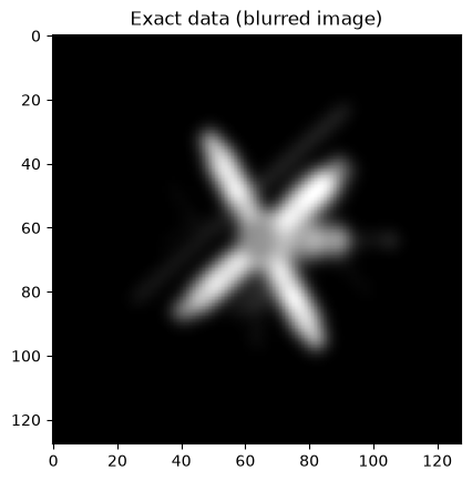
(data2 - probInfo2.exactData).plot()
plt.title("Noise realization");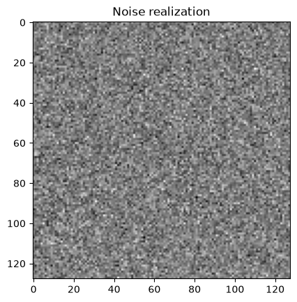
1.2.3. Heat1D: A model for a PDE-based inverse problem
A completely different test problem is The 1D heat test problem, which is described by a partial differential equation (PDE), namely the time-dependent heat equation. The forward model of Heat1D maps an initial temperature distribution on an interval to the temperature distribution after a specified amount of time has passed, by solving the 1D heat equation. For more details, see this specific notebook on PDEs.
Here, we simply set up the test problem in the same way as before:
testproblemH = cuqi.testproblem.Heat1D()
modelH, dataH, probInfoH = testproblemH.get_components()
We start by plotting the exact solution, i.e., the true initial temperature distribution over the interval:
probInfoH.exactSolution.plot()
plt.title("Exact Solution (temperature)");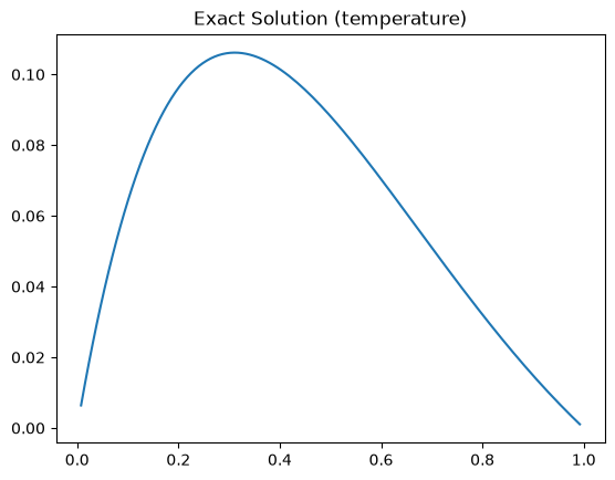
The data is the noisy observations of the temperature distribution after some time has passed (notice the difference in y-axis values). We plot the data and the exact data as well as their difference:
dataH.plot(label="Data (final noisy temperature)")
probInfoH.exactData.plot(label="Exact data (final temperature)")
plt.legend()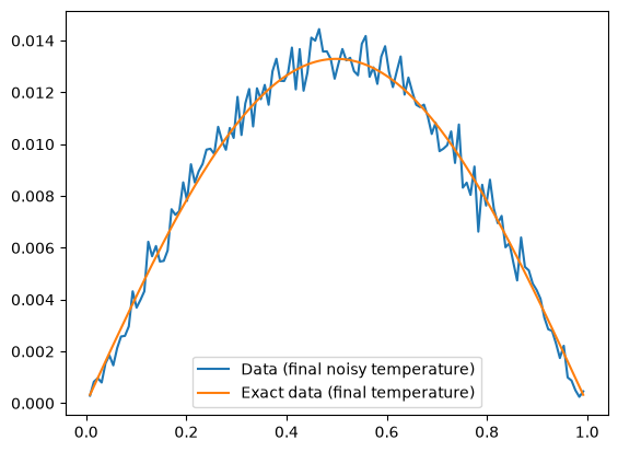
(dataH - probInfoH.exactData).plot()
plt.title("Noise realization");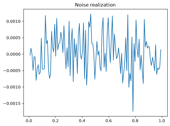
We can take a closer look at the model:
print(modelH)CUQI PDEModel: Continuous1D[128] -> Continuous1D[128].
Forward parameters: ['x'].
PDE: TimeDependentLinearPDE.
Here the domain and range are parametrized as Continuous1D with 128 parameters, and the model is now noted as PDEModel and a new field for a PDE is listed.
A PDEModel in CUQIpy is a model where in each forward computation a PDE is 1) assembled, 2) solved and 3) observed. The specifics would depend on the underlying PDE. With that in mind, let us have a look at the underlying PDE for this PDEModel.
modelH.pdeCUQI TimeDependentLinearPDE.
PDE form expression:
def PDE_form(IC, t): return (Dxx, np.zeros(N), IC)Here we see that the underlying PDE is a time-dependent linear PDE which makes sense for the 1D heat test problem. We could keep exploring PDEModels, but we leave that to our specific notebook on PDEs.
For now, the main message is that the CUQIpy model provides an abstract representation of a forward model of many and different inverse problems, and that CUQIpy offers a collection of test problems containing forward models, data and exact solutions that can be used for demonstration and benchmarking.
1.3. Basic usage of models 
In this section, we demonstrate common operations with CUQIpy models. Let us focus on the LinearModel representing the convolution operation from the deconvolution test problem.
We name the CUQIpy model representing the convolution operator A (recall that A here is not a matrix but a CUQIpy LinearModel) and name the exact solution x_exact.
A, _, probInfo = cuqi.testproblem.Deconvolution1D(dim=64, phantom="sinc").get_components()
x_exact = probInfo.exactSolution
One of the most basic usages of a CUQIpy model is to apply the forward map on some input paramter. This can be simply done by calling the .forward method, or in the case of a LinearModel the short-hand “@” (matrix multiply in Python) can also be used.
y_exact  = A.forward(x_exact) # Explicitly call the forward method
y_exact  = A@x_exact          # Can also use short-hand for matrix multiply (gives the same result)
Linear model also supports basic operations such as evaluating the adjoint, which can also be done using the numpy-like syntax “.T” for transpose. For example here we apply the adjoint operator of A to y_exact.
z = A.adjoint(y_exact) # Explicitly call the adjoint method
z = A.T@y_exact        # Can also use short-hand for matrix transpose (gives the same result)
Unlike Distribution or CUQIarray objects, which have only one geometry attribute, forward models are distinct in having two geometries. domain_geometry relates to the domain of the forward map, and range_geometry relates to the range. These geometries play an important role in linking samplers, which operate on and produce samples in vector form, with forward models, which are geared towards handling more complex data structures. For more discussion on geometries in CUQIpy, please refer to this specific notebook on this topic.
For example, let us take a look at the range geometry of A:
A.range_geometryContinuous1D[64]When computing the forward operation, A passes its range geometry to the output. We can validate this by inspecting y_exact from earlier.
y_exact.geometryContinuous1D[64]This allows plotting in the correct geometry immediately after forward computation
y_exact.plot();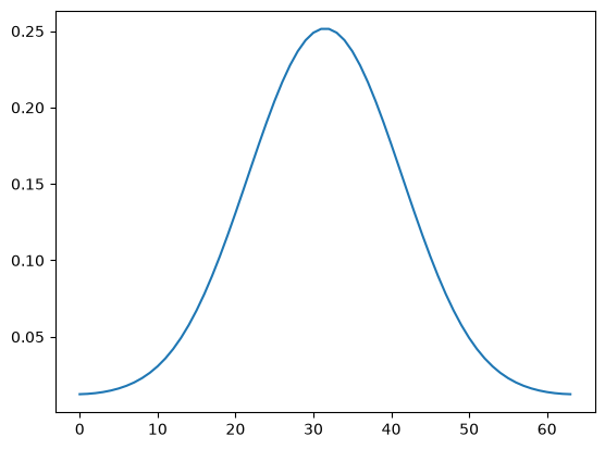
It can be useful to change to domain or range geometries of a model, for example to work with different parametrizations or simply for visualization purposes.
Here we change the range geometry of the model to Discrete and see this reflected in the plotting of the computed output:
A.range_geometry = cuqi.geometry.Discrete(A.range_dim)
A.forward(x_exact).plot()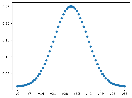
Note that since we are only interested in generating a plot here, we do not need to store a new variable for y_exact, but rather just immediately call the plot method in the same line.
Here we also used A.range_dim to get not the range geometry but the dimension of it. Similarly, we can ask for the dimension of the domain geometry:
A.domain_dim64Some LinearModel objects simply contain a matrix representing the linear mapping; while others use a matrix-free approach. In both cases, one can extract the matrix of the linear model by (this will raise an error if the model is too large):
A.get_matrix()<Compressed Sparse Column sparse matrix of dtype 'float64'
with 4096 stored elements and shape (64, 64)>Finally, models can also be applied to Samples objects, for example to evaluate the forward on all samples. This can be used for forward UQ as shown in Section 5 of this notebook.
Given a distribution and some samples generated from it:
x = cuqi.distribution.Gaussian(np.zeros(A.domain_dim), cov=1)xs = x.sample(1000)
print(type(xs))
xs.shape<class 'cuqi.samples._samples.Samples'>
(64, 1000)i.e. 1000 samples each of size 64 matching the domain of A. We can apply A directly to the Samples object:
ys = A@xsWe plot a couple of selected samples from x:
xs.plot([100,200,300])
plt.title("Samples from x");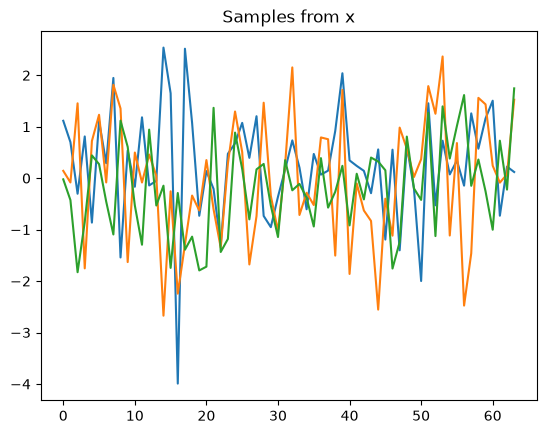
and plot the same samples from y:
ys.plot([100,200,300])
plt.title("Samples from y");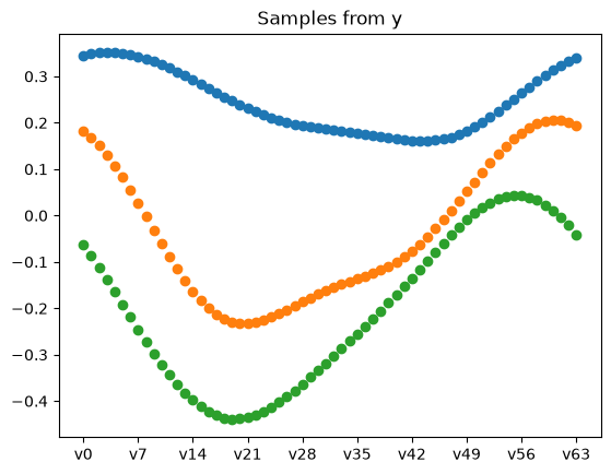
where we note the computed samples ys = A(xs) have the Discrete geometry as A is now equipped with.
# This is where you type the code:
1.4. Generating synthetic data 
Generating synthetic data (potentially many realizations) is a common task when working with inverse problems. In many cases, we want to generate synthetic data to be used in setting up Bayesian inverse problems, for the purpose of testing, verification, and studying various Bayesian model assumptions and solution methods.
In this section, we demonstrate one way this can be achieved by defining the data distribution.
Let us return to the forward model from the deconvolution test problem from earlier, and assume that the measurement data is affected by additive i.i.d. Gaussian noise with standard deviation 0.05. This leads to the Bayesian model for the inverse problem
where , and are random variables and where the goal now is to generate examples of observed data assuming and given some exact solution vector .
Note Generating noisy data in the above example with additive Gaussian noise is rather straightforward. However, the focus here is to provide a common framework for a much larger variety of models and noise types - exemplified by the Gaussian case.
1.4.1. Data distribution
First, note that since is the only random contribution to when is fixed we can directly see that
We call the distribution associated with a data distribution. To generate synthetic data from , we are thus interested in sampling from .
Let us define the model A again and extract the phantom from the probInfo object (just in case some changes were made above):
n = 64
A, _, probInfo = cuqi.testproblem.Deconvolution1D(dim=n, phantom="sinc").get_components()
x_exact = probInfo.exactSolution
The data distribution is conditioned on and so we need to represent a conditional distribution in CUQIpy.
Luckily, when is represented by a CUQIpy model this is easy as we simply provide the model in place of as follows.
y = cuqi.distribution.Gaussian(mean=A, cov=0.05**2)Recall from earlier that the model A had its forward parameter given by ‘x’:
print(A)CUQI LinearModel: Continuous1D[64] -> Continuous1D[64].
Forward parameters: ['x'].
If we now inspect y, we see that it has become a conditional distribution, conditioned on that same ‘x’ parameter.
print(y)CUQI Gaussian. Conditioning variables ['x'].
Note that even though we did not explicitly provide x when defining the mean of y, the object y is able to infer the conditioning on x, since x is the forward parameter of A.
One can be more explicit in specifying the parameter of the forward model by explicitly evaluating the forward model at the desired parameter, provided that this parameter is defined as a distribution. In this way the forward parameter name, x here, can even be changed to another name, e.g. u. First, we define a new distribution u representing the forward parameter:
u = cuqi.distribution.Gaussian(np.zeros(n), cov=1)and using u we can now specify the mean Au:
yu = cuqi.distribution.Gaussian(mean=A@u, cov=0.05**2)
yu
CUQI Gaussian. Conditioning variables ['u'].and we see that u is now the conditioning variable instead of x.
1.4.2. Sampling a data distributions
Evaluating a conditional distribution in CUQIpy is done by use of the “call” method on Python. That is, for a data distribution we would write y(x=x_exact) or simply y(x_exact).
Evaluating the conditional distribution creates a new distribution, where the conditioning variable is fixed. That is, one can think of the expression y(x=x_exact) as defining .
Hence to simulate some noisy data, we just provide the conditioning variable x_exact to the data distribution and then sample.
y_obs = y(x=x_exact).sample()
y_obs.plot();
plt.title("Generated synthetic data");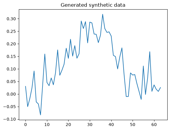
# This is where you type the code:
1.5. Creating custom forward models 
1.5.1. Defining model from a matrix
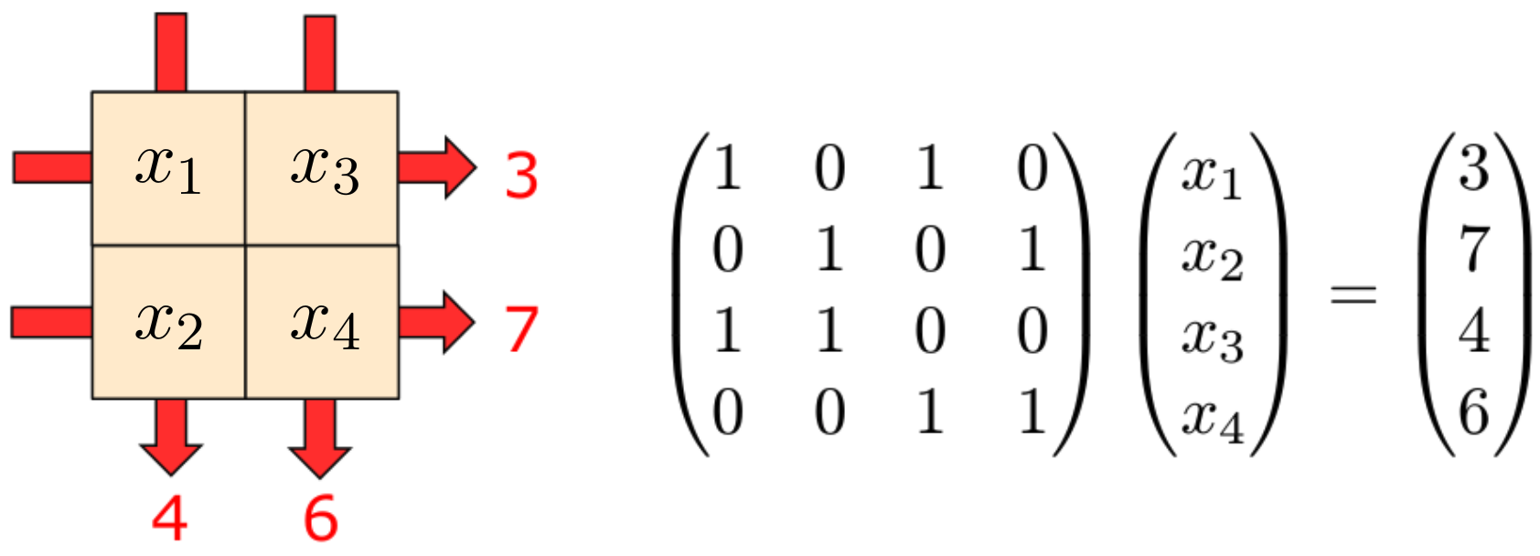
Defining a CUQIpy model from a matrix is easy. Suppose we have the matrix representing the forward operator of the following simple linear inverse problem, which is akin to a sudoko puzzle.
Consider a 2x2 square with unknown pixel values, to be determined from the row and column sums:
#Create a numpy matrix to act like a forward model (this matrix can be replaced to represent other problems)
mat = np.array([
    [1,0,1,0],
    [0,1,0,1],
    [1,1,0,0],
    [0,0,1,1]
])
To create a CUQIpy model represented by this matrix, all we have to do is pass it to the LinearModel class from the model module in CUQIpy as follows.
model_mat = cuqi.model.LinearModel(mat)
print(model_mat)
CUQI LinearModel: _DefaultGeometry1D[4] -> _DefaultGeometry1D[4].
Forward parameters: ['x'].
Here the range and domain geometry is inferred from the matrix. If we want to, we can pass in more explicit information about the range and domain geometries. Here we choose to represent the domain geometry of the four pixel values as a Image2D geometry:
geom1 = cuqi.geometry.Image2D((2,2), order="F", visual_only=True)
geom1Image2D[4]We equip the model with this geometry as the domain geometry:
model_mat.domain_geometry = geom1
model_mat
CUQI LinearModel: Image2D[4] -> _DefaultGeometry1D[4].
Forward parameters: ['x'].When evaluating a CUQIpy model, the domain geometry is used to convert the input from a vector format to what we call a function representation before being evaluated using the user specified map. That is, when we evaluate model_mat, in this case, the Image2D geometry is used to convert the input from a vector format to the 2x2 image before the matrix mat is applied to it. However, mat here expects a vector as an input, so we do not want this default conversion to happen and thus we set visual_only=True, which means the conversion only happens for visualization purposes and not for model evaluation.
To match the order of parameters in the picture above in which and constitutes the first column and and constitutes the second column, we select the column-major order by defining order="F" (F comes from Fortran for historical reasons). This is useful in this case for plotting the solution in the correct order.
Let us create an example 2x2 solution as a CUQIarray equipped with the geometry:
im1 = cuqi.array.CUQIarray([7,5,3,1], geometry=geom1)
im1
CUQIarray: NumPy array wrapped with geometry.
---------------------------------------------
Geometry:
Image2D[4]
Parameters:
True
Array:
CUQIarray([7, 5, 3, 1])which will allow us to display it nicely, even through it is a stored as a vector:
im1.plot()
plt.colorbar()
plt.xticks([]);
plt.yticks([]);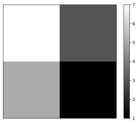
The row and column sum data we can - for the purpose of the example - let be of the type Discrete (labelled) geometry:
geom2 = cuqi.geometry.Discrete(['row1','row2','col1','col2'])We set up and display the observed data from the figure above:
data = cuqi.array.CUQIarray([3,7,4,6], geometry=geom2)
data
CUQIarray: NumPy array wrapped with geometry.
---------------------------------------------
Geometry:
Discrete[4]
Parameters:
True
Array:
CUQIarray([3, 7, 4, 6])data.plot()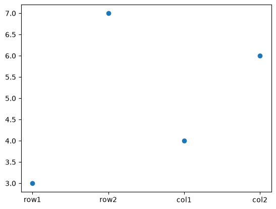
We can equip our model with geom2 as the range geometry:
model_mat.range_geometry = geom2
model_mat
CUQI LinearModel: Image2D[4] -> Discrete[4].
Forward parameters: ['x'].which will allow to apply the forward to an image as if it were a matrix:
data1 = model_mat@im1
data1
CUQIarray: NumPy array wrapped with geometry.
---------------------------------------------
Geometry:
Discrete[4]
Parameters:
True
Array:
CUQIarray([10, 6, 12, 4])Note the resulting data1 automatically has the desired geometry.
We can compare the data computed from im1 against the observed data:
data1.plot()
data.plot(marker="v")
plt.legend(["Observed data", "Data from im1"])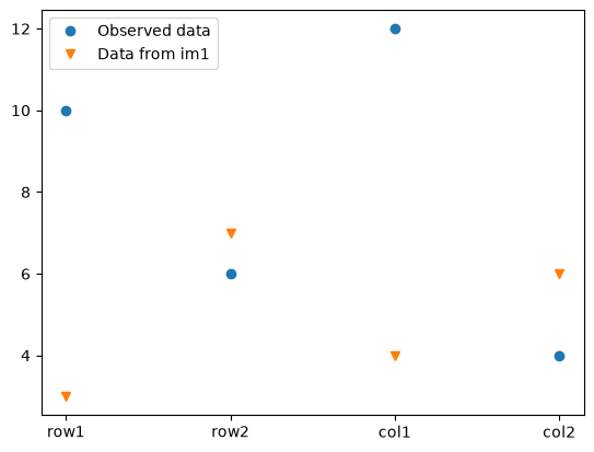
We can also apply the adjoint using matrix transpose notation .T:
adjoint_data = model_mat.T@data1
adjoint_data
CUQIarray: NumPy array wrapped with geometry.
---------------------------------------------
Geometry:
Image2D[4]
Parameters:
True
Array:
CUQIarray([22, 18, 14, 10])and we can visualize the adjoint data (which should be in the domain geometry of A)
adjoint_data.plot()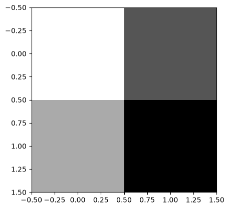
1.5.2. Defining a CUQIpy model from a function
We can also define CUQIpy models from functions. In this case, we must at the minimum provide the dimensions of the range and domain, for example
#This can be any function representing the forward computation. Here just a random function with 3 inputs and 2 outputs
def my_func(x):
    return np.array([x[0]**2+x[1], x[1]+x[2]])
We could provide any geometry of size 2 for the range and size 3 for the domain - here we use the short-hand integer notation to specify uninformative default geometries that only represent the dimension:
model_func = cuqi.model.Model(my_func, range_geometry=2, domain_geometry=3)
print(model_func)
CUQI Model: _DefaultGeometry1D[3] -> _DefaultGeometry1D[2].
Forward parameters: ['x'].
Models will work both on simple numpy arrays and CUQIarrays. Numpy array input will produce numpy array output:
in1 = np.array([3.0, 2.0, 1.0])
out1 = model_func(in1)
print(out1)
type(out1)
[11. 3.]
numpy.ndarrayPassing a CUQIarray input produces a CUQIarray output:
in2 = cuqi.array.CUQIarray(in1)
in2
CUQIarray: NumPy array wrapped with geometry.
---------------------------------------------
Geometry:
_DefaultGeometry1D[3]
Parameters:
True
Array:
CUQIarray([3., 2., 1.])out2 = model_func(in2)
out2CUQIarray: NumPy array wrapped with geometry.
---------------------------------------------
Geometry:
_DefaultGeometry1D[2]
Parameters:
True
Array:
CUQIarray([11., 3.])1.5.3. Linear model from functions
If we have functions for both the forward and adjoint, we can also specify a LinearModel from these functions. Here we illustrate this by creating a forward and adjoint function from the matrix given earlier
def mat_forward(x):
    return mat@x

def mat_adjoint(y):
    return mat.T@y
In this case, the range and domain dimensions (or geometry) cannot be inferred, so they also need to be defined
model_linear_func = cuqi.model.LinearModel(forward=mat_forward,
                                           adjoint=mat_adjoint,
                                           range_geometry=4,
                                           domain_geometry=4)
print(model_linear_func)
CUQI LinearModel: _DefaultGeometry1D[4] -> _DefaultGeometry1D[4].
Forward parameters: ['x'].
The new linear model can then be applied to numpy arrays (or CUQIarrays if including geometries):
z1 = np.array([1., 2., 3., 4.])
z2 = model_linear_func(z1)
z2
array([4., 6., 3., 7.])and the adjoint function is also available:
model_linear_func.T(z2)array([ 7., 9., 11., 13.])- Hansen, P. C. (2010). Discrete Inverse Problems: Insight and Algorithms. SIAM. 10.1137/1.9780898718836