CUQIpy’s Documentation

CUQIpy stands for Computational Uncertainty Quantification for Inverse Problems in python. It’s a robust Python package designed for modeling and solving inverse problems using Bayesian inference. Here’s what it brings to the table:

• A straightforward high-level interface for UQ analysis.

• Complete control over the models and methods.

• An array of predefined distributions, samplers, models, and test problems.

• Easy extendability for your unique needs.

A number of CUQIpy Plugins are available as separate packages that expand the functionality of CUQIpy.

CUQIpy is part of the CUQI project supported by the Villum Foundation.

Quick Links: Installation | Tutorials | How-To Guides | Source Repository | 🔌 CUQIpy Plugins

Getting Started

Get CUQIpy up and running in your machine and learn the basics.

User Guide

Step-by-step tutorials, how-to guide to help you accomplish various tasks with CUQIpy, and in-depth explanations of background theory.

API Reference

Detailed descriptions of CUQIpy library components (modules, classes, methods, etc.).

Contributor’s Guide

Here you find information on how to contribute to CUQIpy. All contributions are welcome, small and big!

🧪 Quick Example - UQ in a few lines of code

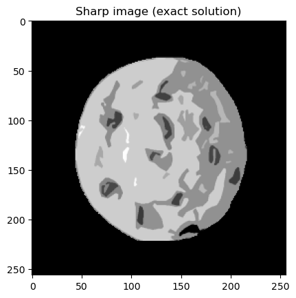
Experience the simplicity and power of CUQIpy with this Image deconvolution example. Getting started with UQ takes just a few lines of code:

# Imports
import matplotlib.pyplot as plt
from cuqi.testproblem import Deconvolution2D
from cuqi.distribution import Gaussian, LMRF, Gamma
from cuqi.problem import BayesianProblem

# Step 1: Set up forward model and data, y = Ax
A, y_data, info = Deconvolution2D(dim=256, phantom="cookie").get_components()

# Step 2: Define distributions for parameters
d = Gamma(1, 1e-4)
s = Gamma(1, 1e-4)
x = LMRF(0, lambda d: 1/d, geometry=A.domain_geometry)
y = Gaussian(A@x, lambda s: 1/s)

# Step 3: Combine into Bayesian Problem and sample posterior
BP = BayesianProblem(y, x, d, s)
BP.set_data(y=y_data)
samples = BP.sample_posterior(200)

# Step 4: Analyze results
info.exactSolution.plot(); plt.title("Sharp image (exact solution)")
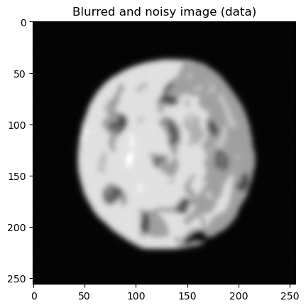
y_data.plot(); plt.title("Blurred and noisy image (data)")
samples["x"].plot_mean(); plt.title("Estimated image (posterior mean)")
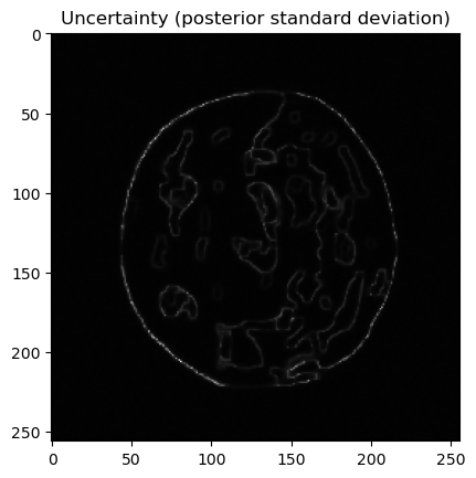
samples["x"].plot_std(); plt.title("Uncertainty (posterior standard deviation)")
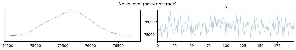
samples["s"].plot_trace(); plt.suptitle("Noise level (posterior trace)")
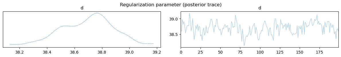
samples["d"].plot_trace(); plt.suptitle("Regularization parameter (posterior trace)")

🔌 CUQIpy Plugins

A number of plugins are available as separate packages that expand the functionality of CUQIpy:

• CUQIpy-CIL: A plugin for the Core Imaging Library (CIL) providing access to forward models for X-ray computed tomography.

• CUQIpy-FEniCS: A plugin providing access to the finite element modelling tool FEniCS, which is used for solving PDE-based inverse problems.

• CUQIpy-PyTorch: A plugin providing access to the automatic differentiation framework of PyTorch within CUQIpy. It allows gradient-based sampling methods without manually providing derivative information of distributions and forward models.

🌟 Contributors

A big shoutout to our passionate team! Discover the talented individuals behind CUQIpy here.