A. Falling object problem - Uncertainty Quantification in Inverse Problems with CUQIpy

This notebook provides the full implementation of the falling object problem discussed in 5. Computational UQ: the need for sampling, which the reader is referred to for more details, particularly on the influence of priors. We demonstrate performing Bayesian inference with CUQIpy on a simple physical model of a falling object with air resistance. We estimate the gravitational acceleration g and the air resistance coefficient C from noisy measurements of the object’s fall distance over time. Our considered problem is a simplified version of that described in Allmaras et al. (2013).

1. Import necessary packages¶

import numpy as np
import matplotlib.pyplot as plt
import cuqi

2. Define forward model and synthetic measurement¶

# Forward model
class FallingObject:
    def __init__(self, t, t0=0.0):
        self.t = np.asarray(t)
        self.t0 = t0

    def __call__(self, x):
        """Analytical solution for a body falling with quadratic air resistance."""
        g, C = x
        v_inf = np.sqrt(g / C)
        tau = self.t - self.t0
        z = (1.0 / C) * np.log(np.cosh(g * tau / v_inf))
        return z

# Parameters
g_true = 9.816 # m/s²  (true gravitational acceleration)
C_true = 0.1 # m⁻¹   (true air resistance coefficient)
t0     = 0.0 # s     (release time)
fps    = 30 # frames per second (as in the paper)

# Simulate ~30 frames after release
n_frames  = 30
frame_ids = np.arange(n_frames)
t_meas    = t0 + frame_ids / fps   # measurement times

# Clean (noise-free) fall distances
falling_object_meas = FallingObject(t_meas, t0)
z_clean = falling_object_meas([g_true, C_true])

noise_std = 0.1
np.random.seed(2026)  # for reproducibility
z_meas = z_clean + noise_std * np.random.randn(len(z_clean))  # Noisy measurements

# Dense trajectory for plotting
t_dense = np.linspace(0.0, t_meas[-1] + 0.05, 500)
falling_object_dense = FallingObject(t_dense, t0)
z_dense = falling_object_dense([g_true, C_true])

fig, ax = plt.subplots(figsize=(4, 3))
ax.plot(t_dense, z_dense, 'k--', linewidth=1.0, label='True trajectory')
ax.plot(t_meas, z_meas, 'o', linewidth=1.0, color='tab:blue', label='Measurements', markersize=3)
ax.set_xlabel('Time (s)')
ax.set_ylabel('Fall distance (m)')
# ax.set_title(f'Measurement with g = {g_true} m/s², C = {C_true} m⁻¹')
ax.legend()
ax.grid(True, alpha=0.3)
ax.invert_yaxis()
plt.tight_layout()
plt.savefig("data.png", dpi=300, bbox_inches='tight')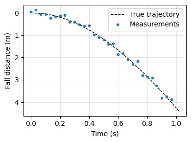

3. Define priors¶

We have three alternatives here:

1. Uniform Prior:

p(\mathbf{x}) = \text{Uniform}(g, C \mid g \in [8, 12], \, C \in [0.01, 0.25])

(1)

2. Truncated Normal Prior:

p(\mathbf{x}) = \mathcal{N}_{\text{trunc}}\left(\boldsymbol{\mu}, \boldsymbol{\Sigma}, \, \mathbf{a}, \mathbf{b}\right)

(2)

where $\boldsymbol{\mu} = [11.0, 0.1]^T$ , $\boldsymbol{\Sigma} = \text{diag}([0.2^2, 0.2^2])$ , $\mathbf{a} = [8.0, 0.01]^T$ , and $\mathbf{b} = [12.0, 0.25]^T$ .

3. Truncated Normal Prior:

p(\mathbf{x}) = \mathcal{N}_{\text{trunc}}\left(\boldsymbol{\mu}, \boldsymbol{\Sigma}, \, \mathbf{a}, \mathbf{b}\right)

(3)

where $\boldsymbol{\mu} = [11.0, 0.1]^T$ , $\boldsymbol{\Sigma} = \text{diag}([2^2, 2^2])$ , $\mathbf{a} = [8.0, 0.01]^T$ , and $\mathbf{b} = [12.0, 0.25]^T$ .

Here, we choose to demonstrate the uniform prior, but the reader can try other prior alternatives by commenting out the uniform prior code and uncommenting the desired prior below.

# 1. Uniform prior
x = cuqi.distribution.Uniform(np.array([8.0, 0.01]), np.array([12.0, 0.25])) # g within [8, 12], C within [0.01, 0.25]
# 2. Truncated normal prior (mean way off the ground truth, but with a small std)
# x = cuqi.distribution.TruncatedNormal(mean=np.array([11.0, 0.2]), std=np.array([0.2, 0.2]), low=np.array([8.0, 0.01]), high=np.array([12.0, 0.25]))
# 3. Truncated normal prior (mean way off the ground truth, and with a large std)
# x = cuqi.distribution.TruncatedNormal(mean=np.array([11.0, 0.2]), std=np.array([2, 2]), low=np.array([8.0, 0.01]), high=np.array([12.0, 0.25]))

4. Define likelihood and posterior¶

A = cuqi.model.Model(falling_object_meas, domain_geometry=2, range_geometry=len(z_meas))

# test A operator
A(x.sample())

# set likelihood and posterior
y = cuqi.distribution.Gaussian(A(x), noise_std**2) # likelihood with Gaussian noise

joint = cuqi.distribution.JointDistribution(y, x)

posterior = joint(y=z_meas) # posterior distribution for given measurements

5. Sample from posterior¶

np.random.seed(1234)  # for reproducibility
sampler = cuqi.sampler.MH(posterior, initial_point=np.array([9.0, 0.1]), scale=0.05)
sampler.warmup(10000)
sampler.sample(20000)
samples = sampler.get_samples().burnthin(10000, 20)

Warmup:   0%|          | 0/10000 [00:00<?, ?it/s, acc rate: 21.05%] /var/folders/6l/nx63qk9s1l7gst1rbgdfb5vc0000gp/T/ipykernel_31607/3367461526.py:10: RuntimeWarning: invalid value encountered in sqrt
  v_inf = np.sqrt(g / C)
Warmup: 100%|██████████| 10000/10000 [00:06<00:00, 1571.88it/s, acc rate: 24.50%]
Sample: 100%|██████████| 20000/20000 [00:14<00:00, 1375.13it/s, acc rate: 23.73%]

samples.plot_trace(exact=np.array([g_true, C_true]))

array([[<Axes: title={'center': 'x0'}>, <Axes: title={'center': 'x0'}>],
       [<Axes: title={'center': 'x1'}>, <Axes: title={'center': 'x1'}>]],
      dtype=object)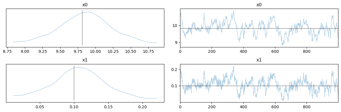

6. Compute MAP¶

from scipy.optimize import minimize, Bounds

# prepare bounds
low = np.asarray(getattr(x, 'low', [8.0, 0.01]), dtype=float).flatten()
high = np.asarray(getattr(x, 'high', [12.0, 0.25]), dtype=float).flatten()
bounds = Bounds(low, high)

def neg_logpost(theta):
    theta = np.asarray(theta, dtype=float)
    return -posterior.logpdf(theta)

# intial guess within bounds
x0 = np.array([10.0, 0.10])

minimize_kwargs = dict(
    fun=neg_logpost,
    x0=x0,
    method='L-BFGS-B',
    bounds=bounds,
    options={'maxiter': 1000, 'ftol': 1e-12, 'gtol': 1e-8},
)

res = minimize(**minimize_kwargs)

map_point = res.x
print("MAP estimate:", map_point)

MAP estimate: [9.86909618 0.10778037]

7. Plots of samples and density¶

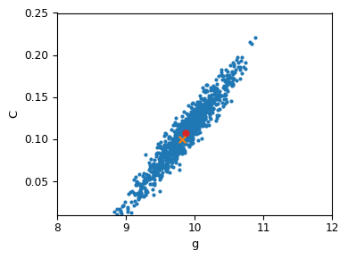
samples.plot_pair(figsize=(4, 3))
plt.scatter(map_point[0], map_point[1], s=100, c="tab:red", marker=".", label="MAP")
plt.scatter(g_true, C_true, s=30, c="tab:orange", marker="x", label="True value")
plt.gca().set_axisbelow(True)
# plt.grid(True, zorder=0)
plt.gca().set_xlabel("g")
plt.gca().set_ylabel("C")
plt.gca().set_xlim(8, 12)
plt.gca().set_ylim(0.01, 0.25)
plt.gca().set_xticks([8, 9, 10, 11, 12])
plt.tight_layout()
plt.savefig("samples.png", dpi=300, bbox_inches='tight')

plt.figure(figsize=(4, 3))  # control figure size here
im = cuqi.utilities.plot_2D_density(
    posterior,
    v1_min=8.0, v1_max=12.0,
    v2_min=0.01, v2_max=0.25,
    N1=200, N2=200
)
plt.scatter(map_point[0], map_point[1], s=100, c="tab:red", marker=".", label="MAP")
plt.scatter(g_true, C_true, s=30, c="tab:orange", marker="x", label="True value")
# plt.grid()
plt.gca().set_aspect('auto')
plt.gca().set_xlabel("g")
plt.gca().set_ylabel("C")
plt.gca().set_xlim(8, 12)
plt.gca().set_ylim(0.01, 0.25)
# plt.colorbar(im)
plt.tight_layout()
plt.savefig("density.png", dpi=300, bbox_inches='tight')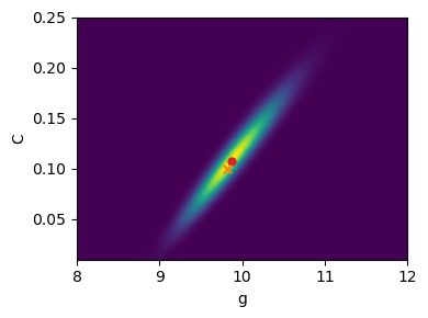

References¶

Allmaras, M., Bangerth, W., Linhart, J. M., Polanco, J., Wang, F., Wang, K., Webster, J., & Zedler, S. (2013). Estimating parameters in physical models through Bayesian inversion: A complete example. SIAM Review, 55(1), 149–167.