Probably the simplest BIP in the world (the short story) - Uncertainty Quantification in Inverse Problems with CUQIpy

Here we define and solve a very simple Bayesian inverse problem (BIP) using CUQIpy. The purpose of this notebook is to introduce the basic concepts of Bayesian inverse problems in a simple way and to use minimal CUQIpy code to solve it.

In the next notebooks (the long story), we discuss more details about setting up this BIP in CUQIpy and provide many exercises to help the reader to explore using CUQIpy in solving BIPs and think of slightly different BIP modeling scenarios.

Contents of this notebook:¶

0. Learning objectives ¶

Create a simple BIP in CUQIpy
- Create a linear forward model object
- Create distribution objects that represent the prior, the noise, and the data distributions
- Use the BayesianProblem class to define the BIP
Solve a simple BIP in CUQIpy
- Compute the maximum a posteriori (MAP) estimate
- Sample from a simple posterior distribution and visualize the results

1. Defining the BIP ¶

Consider the following inverse problem: given observed data $b$ , determine $x_1$ , and $x_2$ :

b = x_1 + x_2 + e \;\;\mathrm{with}\;\; e \sim \mathrm{Gaussian}(0, 0.1)

(1)

We can also write it in the following matrix form:

b = \mathbf{A}\mathbf{x} + e = \large(1,1\large)\binom{x_1}{x_2} + e

(2)

variable	description	dimension
$\mathbf{x}$	parameter to be inferred	2-dimensional
$\mathbf{A}$	forward model	1-by-2 matrix
$b$	data	1-dimensional
$e$	noise	1-dimensional

This problem is:

Considered a linear inverse problem since the forward model is linear.
Ill-posed (in the sense of Hadamard [1]) since the solution is not unique, i.e., for some given value of $b$ , e.g., $b=3$ , all parameter pairs $(x_1, x_2)$ satisfying $x_1 + x_1 = 3$ are solutions to the (noise-free) problem.

Let us define the BIP components and solve it using CUQIpy.

# Importing the required libraries
from cuqi.distribution import Gaussian
from cuqi.problem import BayesianProblem
from cuqi.model import LinearModel
from cuqi.utilities import plot_1D_density, plot_2D_density
import numpy as np
import matplotlib.pyplot as plt

1.1. The forward model ¶

Let us define the forward model $\mathbf{A}$ . We start by specifying the underlying matrix:

A_matrix = np.array([[1.0, 1.0]])

Now we wrap A_matrix in a CUQIpy forward model object, which we name A, as follows:

A = LinearModel(A_matrix)
print(A)

CUQI LinearModel: _DefaultGeometry1D[2] -> _DefaultGeometry1D[1].
    Forward parameters: ['x'].

1.2. The prior ¶

Bayesian approach: Use prior to express belief about solution

A common choice for simplicity is the zero mean Gaussian prior where the components are independent and identically distributed (i.i.d.):

\mathbf{x} \sim \mathrm{Gaussian}(\mathbf{0}, \delta^2 \mathbf{I})

(3)

The probability density function (PDF) of such a Gaussian prior is expressed as

\pi (\mathbf{x}) = \frac{1}{\sqrt{(2 \pi)^n \delta^{2n}}} \mathrm{exp}\left(-\frac{||\mathbf{x}||^2}{2\delta^2}\right)

(4)

where:

$n$ is the dimension of the parameter space (which is 2 in this specific case),
$\delta$ is the standard deviation of the prior distribution,
$\mathbf{I}$ is the identity matrix.

Let us specify the prior distribution for the parameter $\mathbf{x}$ in CUQIpy:

x = Gaussian(np.zeros(2), 2.5)
print(x)

CUQI Gaussian.

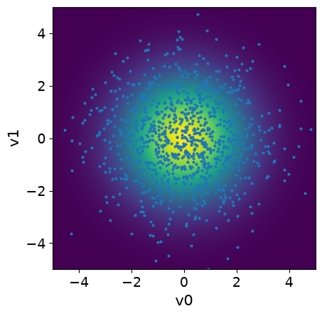
We can plot the prior PDF for the parameters $x_1$ and $x_2$ , along with samples from the prior distribution:

# Plot PDF
plot_2D_density(x, v1_min=-5, v1_max=5, v2_min=-5, v2_max=5)

# Sample
x_samples = x.sample(1000)

# Plot samples
x_samples.plot_pair(ax=plt.gca())
plt.ylim(-5,5);
plt.xlim(-5,5);

1.3. The noise distribution ¶

As mentioned earlier, we assume $e \sim \mathrm{Gaussain}(0, 0.1)$
We can define the noise distribution as follows:

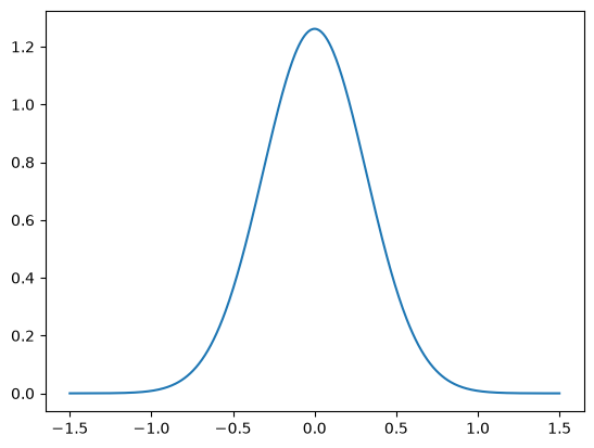
e = Gaussian(0, 0.1)

Let us also plot the PDF of the noise distribution, using the python function plot_pdf_1D:

plot_1D_density(e, -1.5, 1.5)

1.4. The data distribution ¶

The noise in the measurement data follows $e \sim \mathrm{Gaussain}(0, 0.1)$ and due to the relation $b = \mathbf{A}\mathbf{x} + e$ , we can write

b | \mathbf{x} \sim \mathrm{Gaussian}(\mathbf{A}\mathbf{x}, \sigma^2\mathbf{I})

(5)

and in this case we specify $\sigma^2 = 0.1$ .

\pi (b | \mathbf{x}) = \frac{1}{\sqrt{(2 \pi)^m \sigma^{2m}}} \mathrm{exp}\left(-\frac{||\mathbf{A}\mathbf{x}- b||^2}{2\sigma^2}\right)

(6)

The data distribution is the conditional distribution of $b$ given $\mathbf{x}$ .
This PDF can only be evaluated for a given $\mathbf{x}$ .

We create the data distribution object as follows:

b = Gaussian(A@x, 0.1)
print(b)

CUQI Gaussian. Conditioning variables ['x'].

Before sampling or evaluating the PDF of b, we need to specify the value of the parametersx. Let us choose the following value:

particular_x = np.array([1.5, 1.5])

Then we condition the data distribution b on the given parameter particular_x:

b_given_particular_x = b(x=particular_x)
print(b_given_particular_x)

CUQI Gaussian.

Now we have the distribution object b_given_particular_x that represents the data distribution given a particular value of the parameters x. We can now plot the PDF of this distribution:

plot_1D_density(b_given_particular_x, 1.5, 4.5)

We can use b_given_particular_x to simulate noisy data assuming that the true x parameters is particular_x:

b_obs = b_given_particular_x.sample()
print(b_obs)

3.0904619050050224

1.5. The likelihood function ¶

We obtain the likelihood function by fixing observed data $b^\mathrm{obs}$ in the data distribution and considering the function of $\mathbf{x}$ :

L (\mathbf{x} | b^\mathrm{obs}) \mathrel{\vcenter{:}}= \pi (b^\mathrm{obs} | \mathbf{x})

(7)

Since we are using a Gaussian noise model, the likelihood can be evaluated as

L (\mathbf{x} | b=b^\mathrm{obs}) = \frac{1}{\sqrt{(2 \pi)^m \sigma^{2m}}} \mathrm{exp}\left(-\frac{||\mathbf{A}\mathbf{x}- b^\mathrm{obs}||^2}{2\sigma^2}\right) = \frac{1}{\sqrt{2 \pi \cdot 0.1}} \mathrm{exp}\left(-\frac{(x_1+x_2- b^\mathrm{obs})^2}{2\cdot 0.1}\right)

(8)

In CUQIpy, we can define the likelihood function as follows:

likelihood = b(b=b_obs)
print(likelihood)

CUQI Gaussian Likelihood function. Parameters ['x'].

Note that the likelihood function is a density function and is not a distribution. If we try to compute pdf for example, we will get an error.

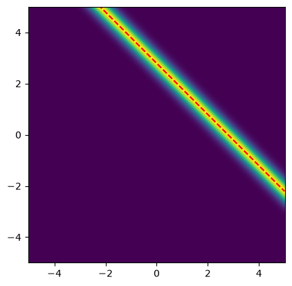
We plot the likelihood function for the observed data b_obs:

x1_lim = np.array([-5, 5])
x2_lim = np.array([-5, 5])
plot_2D_density(
    likelihood,
    v1_min=x1_lim[0], v1_max=x1_lim[1],
    v2_min=x2_lim[0], v2_max=x2_lim[1])

Note: One method of estimating the inverse problem solution is to maximize the likelihood function, which is equivalent to minimizing the negative log-likelihood function. This is known as the maximum likelihood (ML) point estimate.

For this problem, all the points $(x_1, x_2)$ that satisfy $x_1 + x_2 = b^\mathrm{obs}$ are solutions to this maximization problem. These solutions are depicted as the red line in the likelihood plot below.

# Plot the likelihood
plot_2D_density(
    likelihood,
    v1_min=x1_lim[0], v1_max=x1_lim[1],
    v2_min=x2_lim[0], v2_max=x2_lim[1])

# Plot the line x2 = b_obs - x1
plt.plot(x1_lim, b_obs-x1_lim, '--r')
plt.ylim(x2_lim);

Combining the likelihood with the prior will give us a unique maximum a posteriori (MAP) point estimate as we will see next.

1.6. Putting it all together, the BIP ¶

Posterior definition using the Bayes’ rule¶

The posterior is proportional to the product of likelihood and prior

\pi(\mathbf{x} | b=b^\mathrm{obs}) \propto L (\mathbf{x} | b=b^\mathrm{obs}) \pi(\mathbf{x})

(9)

In CUQIpy, we can use the class BayesianProblem to bundle the prior, the data distribution, and the data, then use it to explore the posterior distribution (e.g. point estimate and sampling):

BP = BayesianProblem(b, x)
print(BP)

BayesianProblem with target: 
 JointDistribution(
    Equation: 
	p(b,x) = p(b|x)p(x)
    Densities: 
	b ~ CUQI Gaussian. Conditioning variables ['x'].
	x ~ CUQI Gaussian.
 )

Now we pass the data:

BP.set_data(b=b_obs)
print(BP)

BayesianProblem with target: 
 Posterior(
    Equation:
	 p(x|b) ∝ L(x|b)p(x)
    Densities:
	b ~ CUQI Gaussian Likelihood function. Parameters ['x'].
 	x ~ CUQI Gaussian.
 )

Note the difference in the target of the BayesianProblem object before and after passing the data.

2. Solving the BIP ¶

2.1. Maximum a posteriori (MAP) estimate ¶

Maximizer of the posterior

\mathbf{x}^* = \underset{\mathbf{x}}{\operatorname{argmax\;}} \pi(\mathbf{x} | b=b^\mathrm{obs})

(10)

In the case with Gaussian noise and Gaussian prior, this is the classic Tikhonov solution

\mathbf{x}^* = \underset{\mathbf{x}}{\operatorname{argmin\;}} \frac{1}{2 \sigma^2} ||\mathbf{A}\mathbf{x}- b^\mathrm{obs}||_2^2 + \frac{1}{2\delta^2}||\mathbf{x} ||^2_2

(11)

To compute (and print) the MAP estimate in CUQIpy, we write:

map_estimate = BP.MAP()
print(map_estimate)

!!!!!!!!!!!!!!!!!!!!!!!!!!!!!!!!!!!!!!!!!!!!!!!!!!!!!!!!
!!! Automatic solver selection is a work-in-progress !!!
!!!      Always validate the computed results.       !!!
!!!!!!!!!!!!!!!!!!!!!!!!!!!!!!!!!!!!!!!!!!!!!!!!!!!!!!!!

Using direct MAP of Gaussian posterior. Only works for small-scale problems with dim<=2000.
[1.51493231 1.51493231]

2.2. Sampling from the posterior ¶

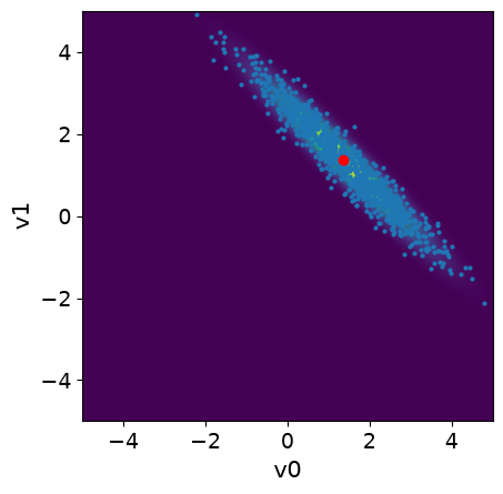
The MAP point is a very useful point estimate, but it does not provide information about the uncertainty associated with the estimate. To quantify this uncertainty, we need to draw samples from the posterior distribution

To sample the posterior distribution in CUQIpy, we can use the sample_posterior method of the BayesianProblem object:

samples = BP.sample_posterior(1000)

!!!!!!!!!!!!!!!!!!!!!!!!!!!!!!!!!!!!!!!!!!!!!!!!!!!!!!!!!!
!!! Automatic sampler selection is a work-in-progress. !!!
!!!       Always validate the computed results.        !!!
!!!!!!!!!!!!!!!!!!!!!!!!!!!!!!!!!!!!!!!!!!!!!!!!!!!!!!!!!!

Using direct sampling of Gaussian posterior. Only works for small-scale problems with dim<=2000.
No burn-in needed for direct sampling.
 Sample 1000 / 1000
Elapsed time: 0.023228168487548828

We visualize the samples:

# Plot the posterior PDF
plot_2D_density(BP.posterior, x1_lim[0], x1_lim[1], x2_lim[0], x2_lim[1])

# Plot the posterior samples
samples.plot_pair(ax=plt.gca())
plt.plot(map_estimate[0], map_estimate[1], 'ro')
plt.ylim(x2_lim);
plt.xlim(x1_lim);

3. Summary ¶

In this notebook, we defined a simple Bayesian inverse problem (BIP) of two unknown parameters and solved it using CUQIpy. We defined the forward model, the prior, and the data distribution; and created simulated data. We then combined these components to define the BIP using the BayesianProblem class. We computed the maximum a posteriori (MAP) estimate and sampled from the posterior distribution to quantify the uncertainty in the estimate.

References ¶

Latz, J. (2020). On the well-posedness of Bayesian inverse problems. SIAM/ASA Journal on Uncertainty Quantification, 8(1), 451-482.