Probably the simplest BIP in the world (the long story) - Uncertainty Quantification in Inverse Problems with CUQIpy

Contents of this notebook:¶

Learning objectives: ¶

Create a linear forward model object in CUQIpy and apply it to some parameters
Create a distribution object in CUQIpy that represents the prior and the noise, and sample, and visualize it
Create and design data distributions in CUQIpy for additive and multiplicative noise case and visualize it
Compute the MAP estimate in CUQIpy
Write the minimization problem that corresponds to finding the MAP estimate
Sample from the posterior distribution in CUQIpy and visualize the samples

The forward model ¶

Consider the following inverse problem: given observed data $b$ , determine $x_1$ , and $x_2$ :

b = x_1 + x_2 + e \;\;\mathrm{with}\;\; e \sim \mathrm{Gaussain}(0, 0.1)

(1)

We can write it as:

b = \mathbf{A}\mathbf{x} + e = \large(1,1\large)\binom{x_1}{x_2} + e

(2)

variable	description	dimension
$\mathbf{x}$	parameter to be inferred	2-dimensional
$\mathbf{A}$	forward model	1-by-2 matrix
$b$	data	1-dimensional
$e$	noise	1-dimensional

This problem is:

Considered a Linear inverse problem since the forward model is linear.
Ill-posed since the solution is not unique (Hadamard 2), i.e., for some given value of $b$ , e.g., $b=3$ , all points $(x_1, x_2)$ that satisfy $x_1 + x_1 = 3$ are solutions to the (noise-free) problem.

# Importing the required libraries
from cuqi.distribution import Gaussian
from cuqi.problem import BayesianProblem
from cuqi.model import LinearModel
import numpy as np
import matplotlib.pyplot as plt
from cuqi.utilities import plot_1D_density, plot_2D_density

/opt/hostedtoolcache/Python/3.11.14/x64/lib/python3.11/site-packages/arviz/__init__.py:50: FutureWarning: 
ArviZ is undergoing a major refactor to improve flexibility and extensibility while maintaining a user-friendly interface.
Some upcoming changes may be backward incompatible.
For details and migration guidance, visit: https://python.arviz.org/en/latest/user_guide/migration_guide.html
  warn(

Let us define the forward model $\mathbf{A}$ , we first define the matrix:

A_matrix = np.array([[1.0, 1.0]])

Verify the dimension of the forward model matrix $\mathbf{A}$

A_matrix.shape

(1, 2)

Now we wrap A_matrix in a CUQIpy forward model object as follows:

A = LinearModel(A_matrix)

Let us test applying the forward model to some parameters:

some_x = np.array([1.0, 2.0])
print(A@some_x)

[3.]

Exercise¶

Try applying A to a different input array
Create a new linear forward model B that represents the identity matrix of dimension 3 and apply it to some parameters
Print both of the models with print(A) and print(B), what do you observe?
Run help(LinearModel) to see the documentation of the class and the input arguments
Is this true for you: “I learned how to create a linear forward model object in CUQIpy and apply it to some parameters.”? If not, what questions do you have?

# your code here

Elaboration on Geometries¶

In CUQIpy, we have the concept of geometries to represent spaces of parameters and data, let us refer to both as variables.

A Geometry object will define the dimension of the space of the variable.
It will define the interpretation of the variable values (e.g. values of function on a 1D or 2D grid, discrete values, coefficients in some expansion, image pixels, etc).
It is equipped with methods of plotting the variables.

We notice that printing the forward model object A, for example, gives us

CUQI LinearModel: _DefaultGeometry1D(2,) -> _DefaultGeometry1D(1,).
    Forward parameters: ['x'].

The first geometry _DefaultGeometry1D(2,) is the domain_geometry which represents the input space of the forward model, i.e., the space of the parameters $x_1$ and $x_2$ .
The second geometry _DefaultGeometry1D(1,) is the range_geometry which represents the output space of the forward model, i.e., the space of the data $b$ .
The forward parameters ['x'] are the parameters that the forward model operates on, in this case, the parameters $x_1$ and $x_2$ .
You can access the domain and range geometries of the forward model object A by A.domain_geometry and A.range_geometry respectively.

print(A.domain_geometry)
print(A.range_geometry)

_DefaultGeometry1D[2]
_DefaultGeometry1D[1]

The _DefaultGeometry1D is a simple geometry that is used as a default geometry in CUQIpy if the user does not specify a geometry.
We will revisit this concept at a later stage depending on forward models needs.

The prior ¶

Bayesian approach: Use prior to express belief about solution¶

A common choice for simplicity is the zero mean Gaussian prior where the components are independent and identically distributed (i.i.d.):

\mathbf{x} \sim \mathrm{Gaussian}(\mathbf{0}, \delta^2 \mathbf{I})

(3)

The probability density function (PDF) of such a Gaussian prior is expressed as

\pi (\mathbf{x}) = \frac{1}{\sqrt{(2 \pi)^n \delta^{2n}}} \mathrm{exp}\left(-\frac{||\mathbf{x}||^2}{2\delta^2}\right)

(4)

where:

$n$ is the dimension of the parameter space (which is 2 in this specific case),
$\delta$ is the standard deviation of the prior distribution,
$\mathbf{I}$ is the identity matrix.

Let us define the prior distribution for the parameters $x_1$ and $x_2$ :

x = Gaussian(np.zeros(2), 2.5)

We can plot the prior PDF for the parameters $x_1$ and $x_2$ :

plot_2D_density(x, -5, 5, -5, 5)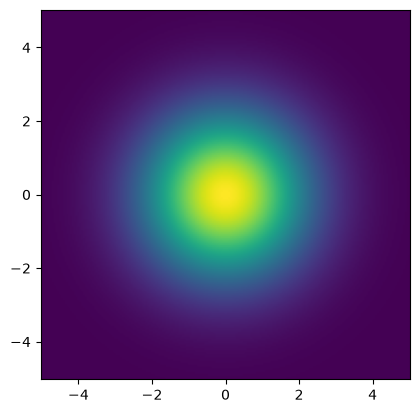

We can sample from the prior distribution:

x_samples = x.sample(1000)

We can visualize the samples from the prior distribution, one way to do this is to plot samples pair plot:

x_samples.plot_pair()

<Axes: xlabel='v0', ylabel='v1'>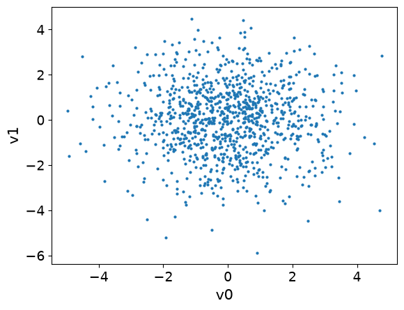

Exercise¶

Can you generate one plot where you visualize the prior PDF and the pair plot together? (tip: after plotting the PDE, you can pass the pyplot current axis to plot_pair method by passing the keyword argument ax=plt.gca())
Does the samples seem to represent the prior distribution correctly?
x_1 and x_2 of the prior distribution are independent and identically distributed random variables. In this exercise: a. Define a new Gaussian distribution x_exercise where x_1 and x_2 are correlated with covariance of 0.7. Set x_1 variance to 1 and x_2 variance to 4 for. The covariance matrix is given by:
$\begin{bmatrix} 1 & 0.7 \\ 0.7 & 4 \end{bmatrix}$
(5)
Visualize the PDF of the new distribution x_exercise and the pair plot of the samples from the distribution in one plot. What do you observe?
Is this true for you: “I learned how to create a distribution object in CUQIpy that represents the prior, sample it, and visualize it”? If not, what questions do you have?

# your code here

The noise distribution ¶

As mentioned earlier, we assume $e \sim \mathrm{Gaussain}(0, 0.1)$
We can define the noise distribution as follows:

e = Gaussian(0, 0.1)

We print the noise distribution object:

print(e)

CUQI Gaussian.

We draw some samples from the noise distribution:

samples = e.sample(10000)

And visualize them. One way to do that is to use the trace plot in CUQIpy:

samples.plot_trace()

array([[<Axes: title={'center': 'v'}>, <Axes: title={'center': 'v'}>]],
      dtype=object)

On the left is a kernel density estimation (KDE) of the samples, and on the right is the trace plot of the samples.

Let us also plot the PDF of the noise distribution, using the python function plot_pdf:

plot_1D_density(e, -1.5, 1.5)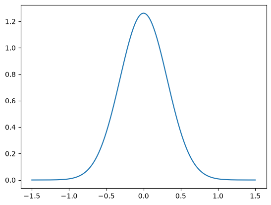

Exercise¶

Create another noise distribution e_exercise with mean 0 and variance 0.5 and plot its PDF
Plot the PDF of the noise distribution e_exercise and the noise distribution e on the same plot
What do you observe?
Is this true for you: “I learned how to create a distribution object in CUQIpy that represents the noise level and visualize it”? If not, what questions do you have?

# your code here

The data distribution ¶

The noise in the measurement data follows $e \sim \mathrm{Gaussain}(0, 0.1)$ and due to the relation $b = \mathbf{A}\mathbf{x} + e$ , we can write

b | \mathbf{x} \sim \mathrm{Gaussian}(\mathbf{A}\mathbf{x}, \sigma^2\mathbf{I})

(6)

and in this case we specify $\sigma^2 = 0.1$ .

\pi (b | \mathbf{x}) = \frac{1}{\sqrt{(2 \pi)^m \sigma^{2m}}} \mathrm{exp}\left(-\frac{||\mathbf{A}\mathbf{x}- b||^2}{2\sigma^2}\right)

(7)

The data distribution is the conditional distribution of $b$ given $\mathbf{x}$ .
This PDF can only be evaluated for a given $\mathbf{x}$ .

We create the data distribution object as follows:

b = Gaussian(A@x, 0.1)

We print the data distribution object:

CUQI Gaussian. Conditioning variables ['x'].

Note that we can not sample from this distribution directly. If we try, we will get an error:

# Here we catch the error and print it
try:
    b.sample(10)
except Exception as e:
    print(e)

Cannot sample from conditional distribution. Missing conditioning variables: ['x']

Before sampling or evaluating the PDF of b, we need to specify the value of the parameters x, let us choose the following value:

particular_x = np.array([1.5, 1.5])

Then we condition the data distribution b on the given parameter particular_x:

b_given_particular_x = b(x=particular_x)

Now we have the distribution object b_given_particular_x that represents the data distribution given a particular value of the parameters x. We can now plot the PDF of this distribution:

plot_1D_density(b_given_particular_x, 1.5, 4.5)

We can use b_given_particular_x to simulate noisy data assuming that the true x parameters is particular_x:

b_obs = b_given_particular_x.sample()
print(b_obs)

3.3048091492383063

Exercise¶

Print the distribution object b_given_particular_x, how does the output differ from printing b.
What is the ratio of the noise in the data (the noise in b_obs) to the true data.
Explain how the data distribution is different from the noise distribution.
Assume we have a multiplicative noise case in which the level of the noise depends on the model output, i.e., $b = (\mathbf{A}\mathbf{x}) e$ where $e \sim \mathrm{Gaussain}(1, 0.1)$ .
- What is the corresponding data distribution?
- Define the data distribution in CUQIpy and call it b_mult. Plot its PDF (condition on particular_x). Tip: you can use lambda function to define the Gaussian covariance lambda x : 0.1*(A@x)**2.
- Plot the PDF of the data distribution b_mult given x=particular_x.
- In general, for the given x_particular, how does the noise to the exact data ratio change in the case of b_mult compared to b?
- Plot the PDF of the data distribution b_mult given a different value of x=np.array([0.4, 0.3]). What can we say about the noise ratio to the exact data in this case? and why?
Is this true for you: “I learned how to create and design data distributions in CUQIpy and visualize it for a given parameter”? If not, what questions do you have?

# your code here

The likelihood function ¶

Likelihood function: by fixing observed data $b^\mathrm{obs}$ in the data distribution and considering the function of $\mathbf{x}$ :

L (\mathbf{x} | b^\mathrm{obs}) \mathrel{\vcenter{:}}= \pi (b^\mathrm{obs} | \mathbf{x})

(8)

Example, given observed data $b^\mathrm{obs}$

L (x_1, x_2 | b=b^\mathrm{obs}) = \frac{1}{\sqrt{2 \pi \cdot 0.1}} \mathrm{exp}\left(-\frac{(x_1+x_2- b^\mathrm{obs})^2}{2\cdot 0.1}\right)

(9)

In CUQIpy, we can define the likelihood function as follows:

likelihood = b(b=b_obs)
print(likelihood)

CUQI Gaussian Likelihood function. Parameters ['x'].

Note that the likelihood function is a density function and is not a distribution. If we try to compute pdf for example, we will get an error:

try:
    likelihood.pdf(x=particular_x)
except Exception as e:
    print(e)

'Likelihood' object has no attribute 'pdf'

while for example, we can evaluate the pdf for the distribution x:

x.pdf(particular_x)

array([0.02588303])

For the likelihood function, we can evaluate its log-density:

likelihood.logd(x=particular_x)

CUQIarray: NumPy array wrapped with geometry.
---------------------------------------------

Geometry:
 _DefaultGeometry1D[1]

Parameters:
 True

Array:
CUQIarray([-0.23218907])

We plot the likelihood function for the observed data b_obs:

x1_lim = np.array([-5, 5])
x2_lim = np.array([-5, 5])
plot_2D_density(
    likelihood,
    x1_lim[0], x1_lim[1],
    x2_lim[0], x2_lim[1])

Maximum likelihood (ML) point estimate ¶

Equivalently, minimizer of negative log of likelihood
In the case of Gaussian noise is the least-squares solution

\mathbf{x}^* = \underset{\mathbf{x}}{\operatorname{argmin\;}} \frac{1}{2 \sigma^2} ||\mathbf{A}\mathbf{x}- b^\mathrm{obs}||_2^2

(10)

We plot likelihood function again but with line $x_2 = b^{obs}-x_1$ :

# Plot the likelihood
plot_2D_density(
    likelihood,
    x1_lim[0], x1_lim[1],
    x2_lim[0], x2_lim[1])

# Plot the line x2 = b_obs - x1
plt.plot(x1_lim, b_obs-x1_lim, '--r')
plt.ylim(x2_lim)

(-5.0, 5.0)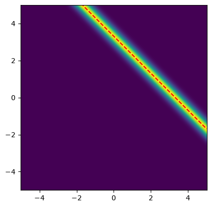

Note that:

All the points on the line $x_2 = b^{obs}-x_1$ have the same likelihood value.
No unique ML point
This is expected, since problem we are solving is: $b^{obs} = x_1 + x_2$
Combining the likelihood with the prior will give us a unique maximum a posteriori (MAP) point estimate as we will see next.

The posterior distribution ¶

Bayes’ rule¶

The posterior is proportional to product of likelihood and prior
$\pi(\mathbf{x} | b) \propto \pi( b|\mathbf{x})\pi(\mathbf{x})$
(11)
Note that $\pi( b|\mathbf{x})$ here denotes the likelihood and not the data distribution, despite often written that way.

In CUQIpy, we can use the class BayesianProblem to bundle the prior, the data distribution, and the data, then use it to explore the posterior distribution (e.g. point estimate and sampling):

BP = BayesianProblem(b, x)
print(BP)

BayesianProblem with target: 
 JointDistribution(
    Equation: 
	p(b,x) = p(b|x)p(x)
    Densities: 
	b ~ CUQI Gaussian. Conditioning variables ['x'].
	x ~ CUQI Gaussian.
 )

Now we pass the data:

BP.set_data(b=b_obs)
print(BP)

BayesianProblem with target: 
 Posterior(
    Equation:
	 p(x|b) ∝ L(x|b)p(x)
    Densities:
	b ~ CUQI Gaussian Likelihood function. Parameters ['x'].
 	x ~ CUQI Gaussian.
 )

Note the difference in the target of the BayesianProblem object before and after passing the data.

Maximum a posteriori (MAP) estimate ¶

Maximizer of the posterior

\mathbf{x}^* = \underset{\mathbf{x}}{\operatorname{argmax\;}} \pi(\mathbf{x} | b)

(12)

In the case with Gaussian noise and Gaussian prior, this is the classic Tikhonov solution

\mathbf{x}^* = \underset{\mathbf{x}}{\operatorname{argmin\;}} \frac{1}{2 \sigma^2} ||\mathbf{A}\mathbf{x}- b^\mathrm{obs}||_2^2 + \frac{1}{2\delta^2}||\mathbf{x} ||^2_2

(13)

Exercise¶

Use the BayesianProblem object to compute the MAP estimate. Objects of the class BayesianProblem have a method MAP that computes the MAP estimate.
Print the solution (the MAP estimate) and compare it to the true solution particular_x, what do you observe? If they are different, why?
Is this true for you: “I learned how to compute the MAP estimate in CUQIpy”? If not, what questions do you have?
Is this true for you: “In paper and pencil, I can write the minimization problem that corresponds to finding the MAP estimate”? If not, what questions do you have?

# your code here

Sampling from the posterior ¶

The MAP point is a very useful point estimate, but it does not provide information about the uncertainty in the estimate. Thus, we need to sample from the posterior distribution to quantify the uncertainty.

Before sampling from the posterior distribution, let us plot the posterior distribution.

Note that in this example the posterior distribution is a multivariate distribution of two parameters only and it is easy to evaluate the PDF of the posterior distribution over a grid of points in the parameter space. However, typically, the posterior distribution is high-dimensional and evaluating the PDF over an n-dimensional grid is not feasible.

plot_2D_density(BP.posterior, x1_lim[0], x1_lim[1], x2_lim[0], x2_lim[1])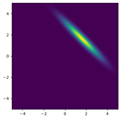

Exercise¶

Use the BayesianProblem object to sample from the posterior distribution. Objects of the class BayesianProblem have a method sample_posterior that samples from the posterior distribution. You can use help(BP.sample_posterior) to see the documentation of the method.
The method sample_posterior returns a Samples object, which is the same type of object that is returned by the sample method of the Distribution class. Visualize the posterior samples using the plot_trace method of the Samples object.
Similar to what you did for the prior, plot the pair plot of the posterior samples over the prior PDF (in the same plot). Are the samples consistent with the posterior distribution PDF?
Is this true for you: “I learned how to sample from the posterior distribution in CUQIpy and visualize the samples”? If not, what questions do you have?

# your code here