2. Distribution gallery - Uncertainty Quantification in Inverse Problems with CUQIpy

In this notebook, we introduce the distribution gallery in CUQIpy: a collection of two-dimensional “toy” distributions provided for illustrative purposes and for testing and benchmarking samplers. Each gallery distribution is specified by its log-density (and gradient) only, making them ideal test targets for the sampling methods covered later in the book. The set follows the benchmark distributions of The Markov-chain Monte Carlo Interactive Gallery.

import numpy as np
import matplotlib.pyplot as plt
import cuqi
from cuqi.distribution import DistributionGallery
from cuqi.sampler import MH, NUTS
np.random.seed(0)

# helper function to plot density of 2D distributions
def plot_2D_density(density, v1_min, v1_max, v2_min, v2_max, N1=201, N2=201,
                    **kwargs):
    """Plot the pdf of a two-dimensional CUQIpy density on a grid."""
    ls1 = np.linspace(v1_min, v1_max, N1)
    ls2 = np.linspace(v2_min, v2_max, N2)
    grid1, grid2 = np.meshgrid(ls1, ls2)

    evaluated_density = np.zeros((N1, N2))
    for ii in range(N1):
        for jj in range(N2):
            logd = density.logd(np.array([grid1[ii, jj], grid2[ii, jj]]))
            evaluated_density[ii, jj] = np.exp(np.squeeze(logd))

    hp_x = 0.5*(v1_max-v1_min)/(N1-1)
    hp_y = 0.5*(v2_max-v2_min)/(N2-1)
    extent = (v1_min-hp_x, v1_max+hp_x, v2_min-hp_y, v2_max+hp_y)
    return plt.imshow(evaluated_density, origin='lower', extent=extent,
                      **kwargs)

# Disable progress bar dynamic update for cleaner output for the book. You can
# enable it again by setting it to True to monitor sampler progress.
cuqi.config.PROGRESS_BAR_DYNAMIC_UPDATE = False

2.1. The gallery at a glance¶

The gallery is loaded through DistributionGallery, which takes the name of the desired distribution as a string. The following distributions are available:

Name	Shape	Useful for testing
`"CalSom91"`	Two crescent-shaped modes	Multimodality with curved modes
`"BivariateGaussian"`	Correlated Gaussian ( $\rho = 0.9$ )	Baseline; the only gallery distribution with direct sampling
`"funnel"`	Neal’s funnel	Distributions whose scale varies strongly across the space
`"mixture"`	Mixture of three Gaussians	Multimodality
`"squiggle"`	Strongly correlated, “squiggly” Gaussian	Strong correlation
`"donut"`	Ring of radius $r$	Non-convex support and strong curvature
`"banana"`	Twisted (“banana-shaped”) Gaussian	Strong curvature; a classic benchmark for HMC-type samplers

All gallery distributions share the same interface: they provide a logpdf (and a gradient), and most of them are density-only — that is, they cannot be sampled directly, only via a sampler.

2.2. Loading a distribution: the “donut”¶

As a first example, we load the “donut” distribution, which is a bivariate distribution of a donut shape. Its log-density is

\begin{aligned} \log(p(\mathbf{x})) \propto - \frac{1}{\sigma_\text{donut}^2} \left( \left\| \mathbf{x} \right\| - r_\text{donut} \right)^2, \end{aligned}

(5)

where $\mathbf{x} = (x_1, x_2)$ is a 2D vector, $\left\| \mathbf{x} \right\|$ is the Euclidean norm of $\mathbf{x}$ , $r_\text{donut}$ is the radius of the donut, and $\sigma_\text{donut}$ is a scalar that controls the width of the “donut”. The density is largest where $\left\| \mathbf{x} \right\| \approx r_\text{donut}$ — i.e. on a ring — and the default parameters are $r_\text{donut} = 2.6$ and $\sigma_\text{donut}^2 = 0.033$ .

target_donut = DistributionGallery("donut")

print(target_donut)

CUQI DistributionGallery.

2.3. Plotting the densities¶

We can visualize the density of a gallery distribution as

plot_2D_density(target_donut, -4, 4, -4, 4)
plt.title("The donut distribution")
plt.show()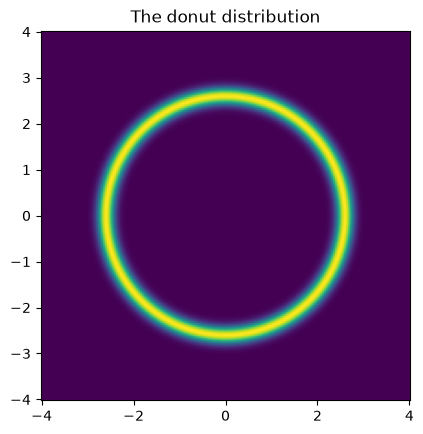

Let’s also plot a few more gallery distributions. Note the different plotting windows needed to capture the mass of each distribution.

for name, window in [("banana", (-5, 5)), ("funnel", (-8, 8)), ("mixture", (-4, 4))]:
    target = DistributionGallery(name)
    plot_2D_density(target, window[0], window[1], window[0], window[1])
    plt.title(f"The {name} distribution")
    plt.show()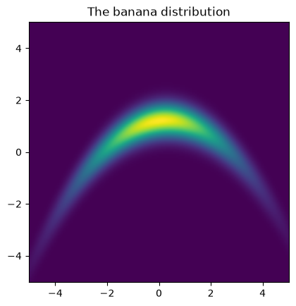

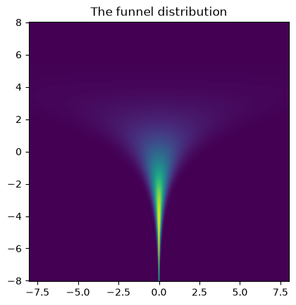
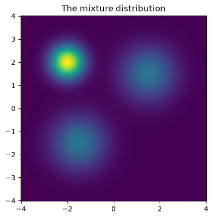
The plots show the variety of shapes in the gallery: the banana is a strongly curved Gaussian, the funnel has a narrow “neck” (the width of $x_1$ varies by orders of magnitude depending on $x_2$ ), and the mixture is clearly multimodal.

2.4. Density and gradient evaluation¶

All gallery distributions provide logpdf and gradient, which is the interface CUQIpy samplers rely on:

x = np.array([2.0, 1.0])
print("logpdf at", x, ":", target_donut.logpdf(x))
print("gradient at", x, ":", target_donut.gradient(x))

logpdf at [2. 1.] : [-4.01353082]
gradient at [2. 1.] : [19.72792101  9.8639605 ]

Note that most gallery distributions do not implement direct sampling (an exception is "BivariateGaussian", which wraps a Gaussian). This is intentional: the gallery targets are meant to be explored with the samplers, which we do next.

target_bivariate = DistributionGallery("BivariateGaussian")
print("BivariateGaussian can be sampled directly:", target_bivariate.sample(3))

BivariateGaussian can be sampled directly: CUQIpy Samples:
---------------

Ns (number of samples):
 3

Geometry:
 _DefaultGeometry1D[2]

Shape:
 (2, 3)

Samples:
 [[ 1.39286824  0.92761334 -0.22646405]
 [ 2.2408932   1.86755799 -0.97727788]]

2.5. Sampling from the gallery¶

Since the gallery targets are density-only, we sample them with CUQIpy samplers. The sampling workflow is: construct the sampler with an initial point, warmup (adapt), then sample, and finally collect the samples with get_samples.

Below we sample the donut distribution with two different samplers: Metropolis–Hastings (MH) with a fixed proposal scale, and the No-U-Turn Sampler (NUTS), which adapts its step size and uses the gradient.

# Metropolis-Hastings with a fixed proposal scale
sampler_mh = MH(target_donut, scale=0.3, initial_point=np.array([3.0, 0.0]))
sampler_mh.warmup(200)
sampler_mh.sample(1000)
samples_mh = sampler_mh.get_samples()

Warmup:   0%|          | 0/200 [00:00<?, ?it/s]

Warmup: 100%|██████████| 200/200 [00:00<00:00, 4861.44it/s, acc rate: 31.50%]

Sample:   0%|          | 0/1000 [00:00<?, ?it/s]

Sample: 100%|██████████| 1000/1000 [00:00<00:00, 4743.20it/s, acc rate: 31.20%]

# NUTS (gradient-based, self-adapting)
sampler_nuts = NUTS(target_donut, initial_point=np.array([3.0, 0.0]))
sampler_nuts.warmup(200)
sampler_nuts.sample(500)
samples_nuts = sampler_nuts.get_samples()

Warmup:   0%|          | 0/200 [00:00<?, ?it/s]

Warmup: 100%|██████████| 200/200 [00:00<00:00, 346.69it/s, acc rate: 64.00%]

Sample:   0%|          | 0/500 [00:00<?, ?it/s]

Sample: 100%|██████████| 500/500 [00:00<00:00, 590.28it/s, acc rate: 70.80%]

# Overlay the samples on the density
plot_2D_density(target_donut, -4, 4, -4, 4)
plt.scatter(samples_mh.samples[0, :200], samples_mh.samples[1, :200],
            s=4, alpha=0.5, color="tab:red", label="MH")
plt.scatter(samples_nuts.samples[0, :200], samples_nuts.samples[1, :200],
            s=4, alpha=0.5, color="tab:blue", label="NUTS")
plt.legend()
plt.title("Samples from the donut distribution")
plt.show()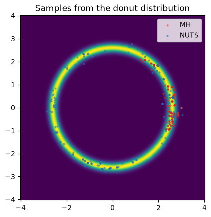

Both samplers correctly concentrate the samples on the ring. The MH sampler with a small fixed step size moves slowly around the ring, while NUTS (which adapts its step size and follows the gradient) explores it more efficiently. The donut is a nice illustration of why the choice of sampler and its tuning parameters matter. For more details on sampling the donut distribution, we refer to 1. Sampling with CUQIpy: five little stories.

2.6. Exercises¶

# your code here