3. Random fields in CUQIpy - Uncertainty Quantification in Inverse Problems with CUQIpy

In many inverse problems, the quantity we want to infer is not a single number but a field, such as an image or a spatially or temporally varying temperature of an object. Such fields are rarely arbitrary: physical quantities tend to vary smoothly, and neighboring values are correlated with each other.

This notebook presents the Gaussian Markov random field (GMRF) in CUQIpy and lists other random fields available in the package. We will briefly explain the intuition behind GMRF and its use within CUQIpy.

3.1. Motivation¶

As a first attempt, consider modeling a field $\mathbf{x} = [x_1, \dots, x_n]^T$ with an i.i.d. Gaussian prior, i.e. each element is independent with the same precision $d$ :

x_i \sim \mathrm{Gaussian}(0, d^{-1}), \qquad \text{independently for } i = 1, \dots, n.

(6)

A sample from this prior looks like white noise:

n = 200
d = 50
x_Gaussian = Gaussian(np.zeros(n), prec=d)

plt.figure(figsize=(10, 3))
x_Gaussian.sample().plot()
plt.title("Sample from $\mathrm{Gaussian}(0, d=50)$")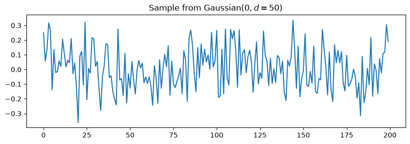

One issue of such a field is that the neighboring values are unrelated. To build correlation into the prior, we need a different construction and this is what the GMRF provides.

3.2. A first look at samples¶

With the same elementwise precision $d = 50$ as the i.i.d. Gaussian above, we define the GMRF prior as follows:

x_GMRF = GMRF(np.zeros(n), d)

Both priors use the same elementwise precision $d = 50$ , so any difference between their samples is due to correlation structure alone. Compare the GMRF sample below with the i.i.d. sample above: it varies smoothly, with neighboring values close together.

plt.figure(figsize=(10, 3))
x_GMRF.sample().plot()
plt.title("Sample from $\mathrm{GMRF}(0, d=50)$")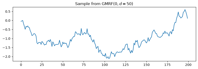

3.3. Definition: the Gaussian Markov random field¶

The key idea of the Markov random field is to put the prior on the differences between neighboring elements rather than on the elements themselves. Particularly in GMRF, we assume that the difference between neighboring elements follows a zero-mean Gaussian with precision $d$ ,

\begin{align*} x_i - x_{i-1} \sim \mathrm{Gaussian}(0, d^{-1}), \quad i=1, \ldots, n, \end{align*}

(7)

This induces a joint Gaussian distribution on $\mathbf{x}$ which we denote by $\mathrm{GMRF}(\mathbf{0}, d)$ — a Gaussian with mean $\mathbf{0}$ and precision $d$ on the neighbor differences. The distribution is implemented in CUQIpy as the GMRF class. For more details on the GMRF, see the CUQIpy paper Riis et al. (2024). The name Markov random field refers to the conditional independence structure of the distribution. For an interior node of our GMRF in 1D, the conditional distribution of $x_i$ given all other nodes is given by

p(x_i \mid x_{j \neq i}) = \mathcal{N}\!\left(\frac{x_{i-1} + x_{i+1}}{2},\; \frac{1}{2d}\right)

(8)

In general, the GMRF defines a zero-mean multivariate Gaussian distribution with precision matrix

\mathbf{P} = d\, \mathbf{D}^T \mathbf{D},

(9)

where $\mathbf{D}$ is the difference matrix. Particularly, the precision matrix $\mathbf{P}$ is tridiagonal: its only non-zero entries lie on the main diagonal and the two adjacent diagonals. This sparsity is particularly attractive computationally and is part of the reason why GMRFs are often used as priors in imaging problems.

3.4. Other Markov random fields in CUQIpy¶

Cauchy Markov Random Field (CMRF): CMRF class
Laplace Markov Random Field (LMRF): LMRF class

CMRF and LMRF are similar to GMRF but with different distributions on the differences between neighboring elements in the signal, where CMRF assumes a Cauchy distribution and LMRF assumes a Laplace distribution. LMRF and CMRF are particularly useful in cases in which the signal to be inferred has sharp edges (jumps). While both LMRF and CMRF favor small differences between neighboring elements, the heavy-tailed LMRF assigns substantially more mass to large differences, making it more suitable when occasional large jumps are expected. Their resulting non-Gaussian posteriors can, however, be more challenging to sample from.

This 1D deconvolution example from Riis et al. (2024) illustrates and compares using the three Markov random fields in a 1D problem.

We have additional approaches to define random fields in CUQIpy through geometry objects. These objects utilize KL expansion to construct random fields with desired correlation properties. For examples on using these fields in inverse problems, we refer the reader to Chapter 13: PDE-based BIP.

Exercises

Can you generate and plot a realization (sample) of x_GMRF? Does the realization show spatial correlation?
Create a Gaussian distribution x_Gaussian with mean np.zeros(n) and precision 50, and compare a sample from the GMRF distribution with the Gaussian distribution by plotting them on the same plot. What do you observe?
★ Generate 100000 samples of x_GMRF and store them in variable x_GMRF_samples. Verify the following about the distribution of the differences. Focus only on verifying the difference between elements 30 and 31 as a representative example.
- The mean of the difference between elements 30 and 31 is close to 0.
- The variance of the difference between elements 30 and 31 is close to $1/50$ .
- Hint: Use this line to create a Samples object of the differences diff_30_31_samples = Samples((x_GMRF_samples.samples[31] - x_GMRF_samples.samples[30]).reshape(1, -1)).

# your code here

References¶

Riis, N. A. B., Alghamdi, A. M. A., Uribe, F., Christensen, S. L., Afkham, B. M., Hansen, P. C., & Jørgensen, J. S. (2024). CUQIpy: I. Computational uncertainty quantification for inverse problems in Python. Inverse Problems, 40(4), 045009. 10.1088/1361-6420/ad22e7