Notebook Cell
from cuqi.distribution import DistributionGallery, Gaussian, JointDistribution
from cuqi.testproblem import Poisson1D
from cuqi.problem import BayesianProblem
import cuqi
import inspect
import numpy as np
import matplotlib.pyplot as plt
from cuqi.sampler import MH, CWMH, ULA, MALA, NUTS
import time
import scipy.stats as sps
from scipy.stats import gaussian_kde
from cuqi.utilities import plot_1D_density

# Disable progress bar dynamic update for cleaner output for the book. You can
# enable it again by setting it to True to monitor sampler progress.
cuqi.config.PROGRESS_BAR_DYNAMIC_UPDATE = False
1.1. The two targets, again
Here we will add the code for building the two targets that we discussed in the previous notebook. The details of the two targets can be found in that notebook. After running the following (hidden) code cell, we will have the two targets ready for sampling:
The donut target
target_donut(distribution)The Poisson 1D target
target_poisson(posterior)
Notebook Cell
# The donut distribution
target_donut = DistributionGallery("donut")

# The Poisson1D Bayesian problem
dim = 201
L = np.pi

xs = np.array([0.2, 0.4, 0.6, 0.8])*L
ws = 0.8
sigma_s = 0.05
def f(t):
    s = np.zeros(dim-1)
    for i in range(4):
        s += ws * sps.norm.pdf(t, loc=xs[i], scale=sigma_s)
    return s

A, _, _ = Poisson1D(dim=dim,
                    endpoint=L,
                    field_type='KL',
                    field_params={'num_modes': 10} ,
                    map=lambda x: np.exp(x),
                    source=f).get_components()
sigma_x = 30
x = Gaussian(0, sigma_x**2, geometry=A.domain_geometry)
np.random.seed(12)
x_true = x.sample()
sigma_y = np.sqrt(0.001)
y = Gaussian(A(x), sigma_y**2, geometry=A.range_geometry)
y_obs = y(x=x_true).sample()
joint = JointDistribution(y, x)
target_poisson = joint(y=y_obs)
In the following (hidden) code cell we define the method plot_pdf_2D for plotting bi-variate PDFs.
Notebook Cell
def plot2d(val, x1_min, x1_max, x2_min, x2_max, N2=201, **kwargs):
    # plot
    pixelwidth_x = (x1_max-x1_min)/(N2-1)
    pixelwidth_y = (x2_max-x2_min)/(N2-1)

    hp_x = 0.5*pixelwidth_x
    hp_y = 0.5*pixelwidth_y

    extent = (x1_min-hp_x, x1_max+hp_x, x2_min-hp_y, x2_max+hp_y)

    plt.imshow(val, origin='lower', extent=extent, **kwargs)
    plt.colorbar()


def plot_2D_density(distb, x1_min, x1_max, x2_min, x2_max, N2=201, **kwargs):
    N2 = 201
    ls1 = np.linspace(x1_min, x1_max, N2)
    ls2 = np.linspace(x2_min, x2_max, N2)
    grid1, grid2 = np.meshgrid(ls1, ls2)
    distb_pdf = np.zeros((N2,N2))
    for ii in range(N2):
        for jj in range(N2):
            distb_pdf[ii,jj] = np.exp(distb.logd(np.array([grid1[ii,jj], grid2[ii,jj]])))
    plot2d(distb_pdf, x1_min, x1_max, x2_min, x2_max, N2, **kwargs)
1.2. Sampling the posterior
After defining the posterior distribution (or a target distribution in general) for the parameters of interest , we can characterize the parameter and its uncertainty by samples from the posterior (target) distribution. However, in general the posterior (target) is not a simple distribution that we can easily sample from. Instead, we need to rely on Markov Chain Monte Carlo (MCMC) methods to sample from the posterior.
In CUQIpy, a number of MCMC samplers are provided in the sampler module that can be used to sample probability distributions. All samplers have the same signature, namely Sampler(target, ...), where target is the target CUQIpy distribution and ... indicates any (optional) arguments.
In CUQIpy we have a number of samplers available, that we can list using:
[sampler for sampler in dir(cuqi.sampler) if not sampler.startswith('_')]['CWMH',
'Conjugate',
'ConjugateApprox',
'Direct',
'HybridGibbs',
'LinearRTO',
'MALA',
'MH',
'MYULA',
'NUTS',
'PCN',
'PnPULA',
'ProposalBasedSampler',
'RegularizedLinearRTO',
'Sampler',
'UGLA',
'ULA']1.2.1. Story 1 - It pays off to adapt: Comparing Metropolis Hastings (MH) with and without adaptation 
In the class, you learned about MH method.
In MH, for each iteration, a new sample is proposed based on the current sample (essintially adding a random perturbation to the corrent sample).
Then the porposed sample is accepted or rejected based on the acceptance probability: , where is the target distribution and is the proposal distribution.
Here we test the MH method with and without adaptation.
For adaptation, MH uses vanishing adaptation to set the step size (scale) to achieve a desired acceptance rate (0.234 in this case).
Let us sample the target_donut with a fixed scale. We first set up the number of samples, number of burn-in samples, and the fixed scale.
Ns = 10000 # Number of samples
Nb = 0 # Number of burn-in samples
scale = 0.05 # Fixed step size "scale"
We create the MH sampler with the target distribution target_donut, the scale scale and an initial sample x0.
MH_sampler = MH(target_donut, scale=scale, initial_point=np.array([0,0]))We sample using sample method:
MH_sampler.sample(Ns+Nb)
MH_fixed_samples = MH_sampler.get_samples().burnthin(Nb)
Sample: 0%| | 0/10000 [00:00<?, ?it/s]Sample: 100%|██████████| 10000/10000 [00:04<00:00, 2417.21it/s, acc rate: 87.42%]
The samples are stored in a Samples object that is returned by the sample method. Let us visualize the samples using the plot_pair method, along with the density of the target distribution using the plot_2D_density method:
plot_2D_density(target_donut, -4, 4, -4, 4)
MH_fixed_samples.plot_pair(ax=plt.gca())
/tmp/ipykernel_2987/1264361712.py:23: DeprecationWarning: Conversion of an array with ndim > 0 to a scalar is deprecated, and will error in future. Ensure you extract a single element from your array before performing this operation. (Deprecated NumPy 1.25.)
distb_pdf[ii,jj] = np.exp(distb.logd(np.array([grid1[ii,jj], grid2[ii,jj]])))
<Axes: xlabel='v0', ylabel='v1'>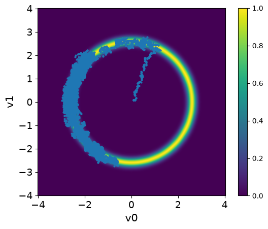
Observations
The samples captures only part of the target distribution.
Once the chain reaches the high density region, it stays there.
The samples starts at the center and takes some time to move to the donut shape. This part of the chain is the burn-in phase.
# your code here
Now we try the solving the same problem with adaptation. We make sure to set the scale to the previous value 0.05.
MH_sampler.scale = 0.05Then we sample this time using sample_adapt method which adapts the step size. Note that the adaptation happen during the burin-in phase so we need to set Nb to some large value to see the effect of adaptation.
Ns = 8500
Nb = 1500
MH_sampler.warmup(Nb)
MH_sampler.sample(Ns)
MH_adapted_samples = MH_sampler.get_samples().burnthin(Nb)
Warmup: 0%| | 0/1500 [00:00<?, ?it/s]Warmup: 100%|██████████| 1500/1500 [00:00<00:00, 4286.06it/s, acc rate: 57.27%]
Sample: 0%| | 0/8500 [00:00<?, ?it/s]Sample: 100%|██████████| 8500/8500 [00:04<00:00, 2104.47it/s, acc rate: 37.07%]
Here we visualize the results (both the ones with and without adaptation). We set the color of the samples and the transparency alpha using the arviz argument scatter_kwargs:
plot_2D_density(target_donut, -4, 4, -4, 4)
MH_fixed_samples.plot_pair(ax=plt.gca(),scatter_kwargs={'c':'b', 'alpha':0.3})
MH_adapted_samples.plot_pair(ax=plt.gca(),scatter_kwargs={'c':'r', 'alpha':0.3})
/tmp/ipykernel_2987/1264361712.py:23: DeprecationWarning: Conversion of an array with ndim > 0 to a scalar is deprecated, and will error in future. Ensure you extract a single element from your array before performing this operation. (Deprecated NumPy 1.25.)
distb_pdf[ii,jj] = np.exp(distb.logd(np.array([grid1[ii,jj], grid2[ii,jj]])))
<Axes: xlabel='v0', ylabel='v1'>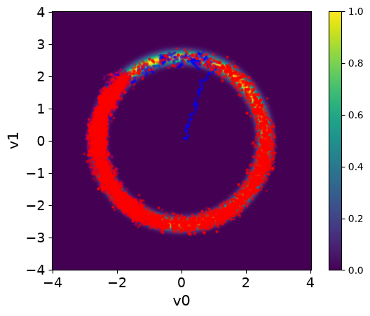
# your code here
Let us plot the chains for the two cases, removing the burin-in from the fixed scale case:
MH_fixed_samples.burnthin(Nb).plot_trace()
MH_adapted_samples.plot_trace()
array([[<Axes: title={'center': 'v0'}>, <Axes: title={'center': 'v0'}>],
[<Axes: title={'center': 'v1'}>, <Axes: title={'center': 'v1'}>]],
dtype=object)

Notes
The chains in the second case (with adaptation) has much better mixing compared to the first case (closer to a fuzzy warm shape).
The estimate density of the target distribution is much better in the second case, captures the 2 modes.
We can also use plot_pair with additional arviz arguments kind, kde_kwargs, and marginals to visualize the marginals and the kernel density estimate of the target distribution. Let us do this for the two cases:
MH_adapted_samples.plot_pair(kind=["scatter", "kde"], kde_kwargs={"fill_last": False}, marginals=True)
MH_fixed_samples.plot_pair(kind=["scatter", "kde"], kde_kwargs={"fill_last": False}, marginals=True)
array([[<Axes: >, None],
[<Axes: xlabel='v0', ylabel='v1'>, <Axes: >]], dtype=object)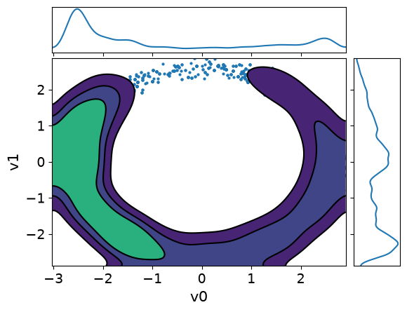
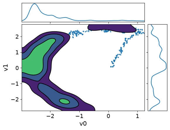
It is clear from these figures how using adaptation of the step size is very beneficial to capture the target distribution in this scenario.
1.2.2. Story 2 - Not all unknowns are created equal: Component-wise Metropolis Hastings CWMH
To get to the next sample, CWMH updates the components of the current sample one at a time and applies the accept/reject step for each component. Updating the scale happens for each component separately depending on the acceptance rate of the component.
Let us test sampling the Poisson problem target with CWMH. We fix the seed for reproducibility and set the number of samples, burn-in samples, and the scale.
np.random.seed(0) # Fix the seed for reproducibility
scale = 0.06
Ns = 500
Nb = 500
For comparison, we sample the Poisson problem target with the MH sampler first:
MH_sampler = MH(target_poisson, scale = scale, initial_point=np.ones(target_poisson.dim))
MH_sampler.warmup(Nb)
MH_sampler.sample(Ns)
MH_samples = MH_sampler.get_samples().burnthin(Nb)
Warmup: 0%| | 0/500 [00:00<?, ?it/s]Warmup: 100%|██████████| 500/500 [00:02<00:00, 244.23it/s, acc rate: 51.20%]
Sample: 0%| | 0/500 [00:00<?, ?it/s]Sample: 100%|██████████| 500/500 [00:01<00:00, 275.21it/s, acc rate: 46.60%]
Then we create a CWMH sampler with the target distribution target_poisson, the scale scale and an initial sample x0 and sample from it.
CWMH_sampler = CWMH(target_poisson, scale = scale, initial_point=np.ones(target_poisson.dim))
CWMH_sampler.warmup(Nb)
CWMH_sampler.sample(Ns)
CWMH_samples = CWMH_sampler.get_samples().burnthin(Nb)
Warmup: 0%| | 0/500 [00:00<?, ?it/s]Warmup: 100%|██████████| 500/500 [00:36<00:00, 13.61it/s, acc rate: 82.90%]
Sample: 0%| | 0/500 [00:00<?, ?it/s]Sample: 100%|██████████| 500/500 [00:12<00:00, 41.27it/s, acc rate: 90.58%]
Note that we use adaptation in both cases. Let us visualize the credible intervals in both cases: for MH
MH_samples.plot_ci(exact=x_true)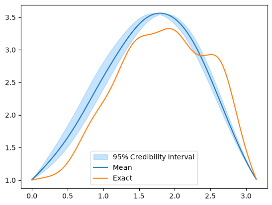
And for CWMH
CWMH_samples.plot_ci(exact=x_true)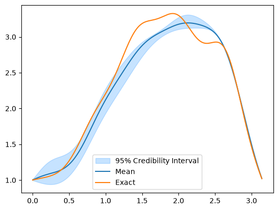
# your code here
1.2.3. Story 3 - May the force guide you: Unadjusted Langevin algorithm (ULA)
In the Unadjusted Langevin algorithm (ULA), new states are proposed using (overdamped) Langevin dynamics.
Let denote a probability density on , from which it is desired to draw an ensemble of i.i.d. samples. We consider the overdamped Langevin Itô diffusion
driven by the time derivative of a standard Brownian motion and force given as gradient of a potential .
In the limit, as , the probability distribution of approaches a stationary distribution, which is also invariant under the diffusion. It turns out that this distribution is .
Approximate sample paths of the Langevin diffusion can be generated by the Euler--Maruyama method with a fixed time step . We set and then recursively define an approximation to the true solution by
where each .
Let us create the ULA sampler in CUQIpy with the target distribution target_donuts, a fixed scale scale, and an initial sample x0:
ULA_sampler = ULA(target=target_donut, scale=0.065, initial_point=np.array([0,0]))We set the number of samples, and sample the target distribution using the sample method:
Ns = 1000
ULA_sampler.sample(Ns)
ULA_samples = ULA_sampler.get_samples()
Sample: 0%| | 0/1000 [00:00<?, ?it/s]Sample: 100%|██████████| 1000/1000 [00:00<00:00, 8517.46it/s, acc rate: 100.00%]
And visualize the samples using the plot_pair method:
plot_2D_density(target_donut, -4, 4, -4, 4)
ULA_samples.plot_pair(ax=plt.gca(), scatter_kwargs={'alpha': 1})
/tmp/ipykernel_2987/1264361712.py:23: DeprecationWarning: Conversion of an array with ndim > 0 to a scalar is deprecated, and will error in future. Ensure you extract a single element from your array before performing this operation. (Deprecated NumPy 1.25.)
distb_pdf[ii,jj] = np.exp(distb.logd(np.array([grid1[ii,jj], grid2[ii,jj]])))
<Axes: xlabel='v0', ylabel='v1'>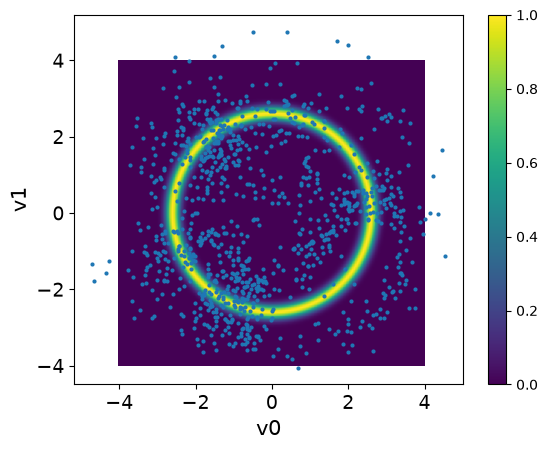
We note that the samples are all over the domain and do not capture the target distribution. This is because the ULA sampler will result in approximate (biased) distribution that as will converge to .
# your code here
1.2.4. Story 4: This is a bias we can fix - Metropolis-adjusted Langevin algorithm (MALA)
In contrast to the Euler--Maruyama method for simulating the Langevin diffusion. MALA incorporates an additional step. We consider the above update rule as defining a proposal for a new state:
this proposal is accepted or rejected according to the MH algorithm.
That is, the acceptance probability is:
where the proposal has the form
The combined dynamics of the Langevin diffusion and the MH algorithm satisfy the detailed balance conditions necessary for the existence of a unique, invariant, stationary distribution.
For limited classes of target distributions, the optimal acceptance rate for this algorithm can be shown to be 0.574; this can be used to tune .
Let us get back to the uni-variate Gaussian target distribution x_uni that was suggested in the exercise of the previous section. We saw that when the scale was 1, the resulting samples did not capture the target distribution, but an appreciably different one, which shows the bias in ULA.
We will now use MALA to sample from this target distribution. Let us create x_uni first:
x_uni = Gaussian(0, 1)Then we create a MALA sampler object MALA_uni for the target distribution x_uni with scale 1 and initial sample 0 and sample from it:
MALA_uni = MALA(x_uni, scale=1, initial_point=0)

Ns = 40000
MALA_uni.sample(Ns)
ULA_samples_uni = MALA_uni.get_samples()
Sample: 0%| | 0/40000 [00:00<?, ?it/s]Sample: 100%|██████████| 40000/40000 [00:35<00:00, 1118.04it/s, acc rate: 92.12%]
Lastly, we visualize the KDE obtained from samples along with the target distribution PDF:
plot_1D_density(x_uni, -4, 4, label='True')
grid = np.linspace(-4, 4, 1000)
kde_est = gaussian_kde(ULA_samples_uni.samples[0,:])
plt.plot(grid, kde_est(grid), label='Estimated')
plt.legend()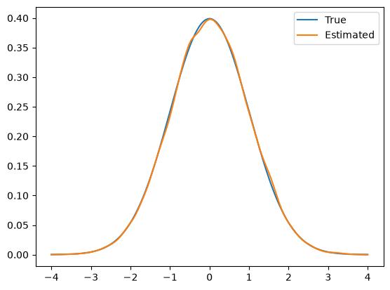
We notice in this case that the KDE of the samples captures the target distribution well. This is because MALA corrects the bias in ULA by using the MH acceptance step.
1.2.5. Story 5 - Sampling goes nuts with NUTS: Hamiltonian Monte Carlo (HMC) and No-U-Turn Sampler (NUTS)
Hamiltonian Monte Carlo (HMC): use Hamiltonian dynamics to simulate particle trajectories.
Define a Hamiltonian function in terms of the target distribution.
Introduce an auxiliary momentum variables, which typically have independent Gaussian distributions.
Hamiltonian dynamics operate on a -dimensional position vector , and a -dimensional momentum vector , so that the full state space has dimensions. The system is described by a function of and known as the Hamiltonian .
In HMC, one uses Hamiltonian functions that can be written as (closed-system dynamics):
The potential energy is completely determined by the target distribution, indeed is equal to the logarithm of the target distribution .
The kinetic energy is unconstrained and must be specified by the implementation.
The Hamiltonian is an energy function for the joint state of position-momentum, and so defines a joint distribution for them as follows:
There are several ways to set the kinetic energy (density of the auxiliary momentum):
Euclidean--Gaussian kinetic energy: using a fixed covariance estimated from the position parameters, .
Riemann--Gaussian kinetic energy: unlike the Euclidean metric, varies as one moves through parameter space, .
Non-Gaussian kinetic energies.
Hamilton’s equations read as follows:
where is the gradient of the logarithm of the target density.
Discretizing Hamilton’s equations:
Symplectic integrators: the leapfrog method (the standard choice).
Hamiltonian dynamics are time-reversible and volume-preserving.
The dynamics keep the Hamiltonian invariant. A Hamiltonian trajectory will (if simulated exactly) move within a hypersurface of constant probability density.
Each iteration of the HMC algorithm has two steps. Both steps leave the joint distribution of invariant (detailed balance).
In the first step, new values of are randomly drawn from their Gaussian distribution, independently of the current .
In the second step, a Metropolis update is performed, using Hamiltonian dynamics to propose a new state.
Optimal acceptance rate is 0.65. The step size and trajectory length need to be tuned.
No-U-Turn sampler
HMC is an algorithm that avoids the random walk behavior and sensitivity to correlated parameters that plague many MCMC methods by taking a series of steps informed by first-order gradient information.
However, HMC’s performance is highly sensitive to two user-specified parameters: a step size and a desired number of steps .
The No-U-Turn Sampler (NUTS), an extension to HMC that eliminates the need to set a number of steps , as well as the step-size.
We simulate in discrete time steps, and to make sure you explore the parameter space properly you simulate steps in one direction and the twice as many in the other direction, turn around again, etc. At some point you want to stop this and a good way of doing that is when you have done a U-turn (i.e., appear to have gone all over the place).
NUTS begins by introducing an auxiliary variable with conditional distribution. After re-sampling from this distribution, NUTS uses the leapfrog integrator to trace out a path forwards and backwards in fictitious time. First running forwards or backwards 1 step, then forwards or backwards 2 steps, then forwards or backwards 4 steps, etc.
This doubling process implicitly builds a balanced binary tree whose leaf nodes correspond to position-momentum state. The doubling is stopped when the subtrajectory from the leftmost to the rightmost nodes of any balanced subtree of the overall binary tree starts to double back on itself (i.e., the fictional particle starts to make a U-turn).
At this point NUTS stops the simulation and samples from among the set of points computed during the simulation, taking care to preserve detailed balance.
To adapt the step-size, NUTS uses a modified dual averaging algorithm during the burn-in phase.
The good thing about NUTS is that proposals are made based on the shape of the posterior and they can happend at the other end of the distribution. In contrast, MH makes proposals within a ball, and Gibbs sampling only moves along one (or at least very few) dimensions at a time.
Let us try the NUTS sampler in CUQIpy for the donut target distribution target_donut. We create the NUTS sampler object NUTS_donut for the target distribution target_donut with initial sample [0, 0]:
NUTS_donut = NUTS(target=target_donut, initial_point=np.array([0,0]))We set the number of samples and burin-in and sample the target distribution: Note: for NUTS in CUQIpy, using sample or sample_adapt is the same. NUTS will always adapt if the number of burn-in samples is larger than 0 and the parameter adapt_step_size is passed as True, the later is a default behavior.
Ns = 100
Nb = 10
NUTS_donut.warmup(Nb)
NUTS_donut.sample(Ns)
NUTS_donuts_samples = NUTS_donut.get_samples().burnthin(Nb)
Warmup: 0%| | 0/10 [00:00<?, ?it/s]Warmup: 100%|██████████| 10/10 [00:00<00:00, 1218.57it/s, acc rate: 70.00%]
Sample: 0%| | 0/100 [00:00<?, ?it/s]Sample: 100%|██████████| 100/100 [00:00<00:00, 678.30it/s, acc rate: 81.00%]
Let us visualize the samples using the plot_pair method over the target distribution PDF. We will also add connetions between the samples to visualize the path of the NUTS sampler:
plot_2D_density(target_donut, -4, 4, -4, 4)
NUTS_donuts_samples.plot_pair(ax=plt.gca(), scatter_kwargs={'alpha': 1, 'c': 'r'})
plt.plot(NUTS_donuts_samples.samples[0,:], NUTS_donuts_samples.samples[1,:], 'r', alpha=0.5)
/tmp/ipykernel_2987/1264361712.py:23: DeprecationWarning: Conversion of an array with ndim > 0 to a scalar is deprecated, and will error in future. Ensure you extract a single element from your array before performing this operation. (Deprecated NumPy 1.25.)
distb_pdf[ii,jj] = np.exp(distb.logd(np.array([grid1[ii,jj], grid2[ii,jj]])))
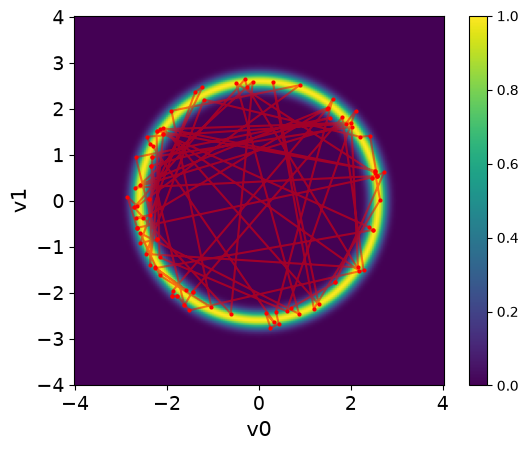
We can see that NUTS can take rapid steps in exploring the target distribution. The samples are spread all over the domain and capture the target distribution efficiently.
# your code here# your code here
np.random.seed(0) # Fix the seed for reproducibility
We see that although the number of NUTS samples is much smaller than in the CWMH samples, the ESS is much larger. This however comes at a cost of computational time, which is due to building the tree structure in each iteration as well as the finite difference approximation of the gradient. Note that other approaches that are more computationally efficient can be used to compute the gradient of the target distribution, e.g. computing the adjoint-based gradient.